Wing Problem
The Wing problem provides an interface for generating aerodynamic datasets for wings using high-fidelity computational fluid dynamics (CFD) workflow. Users can parameterize wing planform parameters, wing airfoil cross-section, flow conditions, and evaluate the resulting configurations without manually setting up the geometry, meshing, solver, and post-processing workflow. The Wing problem currently uses ADflow as the CFD solver and the OpenVSP for wing shape parameteriation. Additional CFD solvers, such as OpenFOAM and SU2, may be supported in future releases. The following sections describe the dependencies, computational workflow, and how to generate aerodynamic datasets with the Wing problem.
Dependencies
The Wing problem requires several additional packages that must be installed before using this problem. The required packages and their corresponding versions are listed below.
Package |
Version |
Comments |
|---|---|---|
3.1.6 |
Used for parallel processing during mesh deformation and CFD solver execution |
|
- |
Used for monitoring child processes launched for analysis |
|
>= 1.8.4 |
Provides |
|
- |
Handles wing shape paramerization |
|
>= 1.17.0 |
Provides an interface for handling wing shape parameterization through OpenVSP |
|
>= 2.6.2 |
Used for morphing volume mesh based on given shape parameters |
|
2.11.0 |
Used as the CFD solver for wing flow simulations |
|
- |
Used for reading, processing, and writing surface and volume field data |
|
- |
Used for creating and storing field results in HDF5 format |
Make sure that all required packages are installed with compatible versions before using the Wing problem.
Workflow
The Wing problem accepts a set of samples, where each sample contains parameter values. This set may contain a single sample or multiple samples. For each sample \(x_i\) in the sample set, the Wing problem performs the sequence of operations described below:
Wing shape parameterization: The geometry parameters are used to define the wing planform shape and airfoil cross-section through OpenVSP and pyGeo
Volume mesh deformation: A baseline volume mesh is deformed based on the wing geometry using
idwarpCFD analysis: The deformed volume mesh and the flow parameters are passed to the
ADflowsolver to compute aerodynamic solutionOutput extraction: Scalar and field quantities from the solver are extracted and stored in a folder
When multiple samples are provided, the workflow is evaluated for each sample, and the resulting outputs are stored separately for each sample. This allows the Wing problem to provide a consistent interface for generating datasets without requiring users to manually manage geometry processing, mesh deformation, solver execution, or output handling.
The complete workflow is illustrated in the XDSM diagram below.
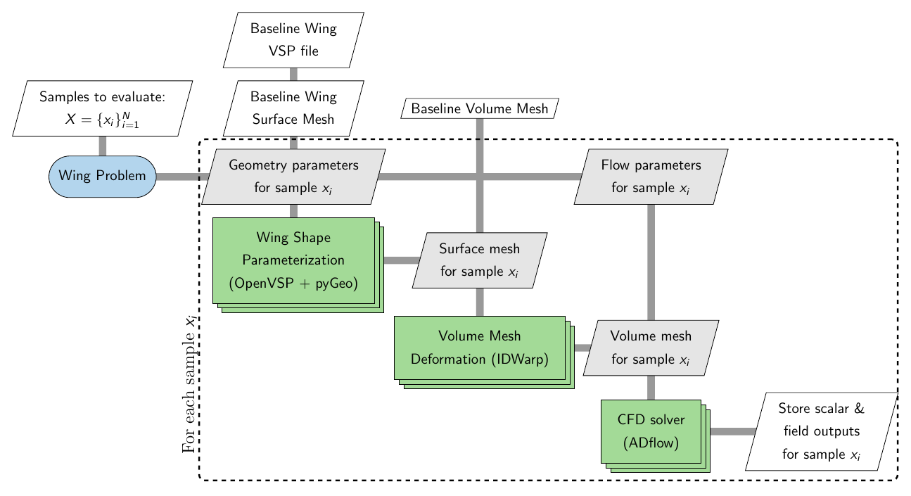
The stacked rectangles representing the shape paramerization, volume mesh deformation, and CFD analysis indicate that these operations use multiple processors through MPI. The Wing problem therefore abstracts the geometry processing, mesh deformation, solver execution, and output handling required for each sample.
Basic usage
To use the Wing problem, you will require a baseline volume mesh in CGNS format. The Wing problem does not generate a volume mesh from the wing planform, rather the shape changes are transferred to the volume mesh using pyGeo and idwarp. It is recommended to check that this baseline volume mesh works with ADFlow solver. Along with the volume mesh, you will need an OpenVSP model file (.vsp3) that describes the baseline wing planform and geometry around which the volume mesh is created.
Note
An OpenVSP model file is only required if you want to modify the wing shape
It is important to keep in mind the following guidelines while creating OpenVSP model:
The OpenVSP model must contain exactly one component of type
WINGUse span, root chord, and tip chord triplet to define the wing planform, you can only modify these three quantities.
Additionally, if you are planning to modify the cross-section airfoil, then keep in mind the following things:
Set the airfoil type to
CST_AIRFOIL, currently you can only modify the airfoil shape using CST methodTrim the trailing edge at each cross-section using an appropraite value relative to the local chord. It is important to use a relative value to avoid collapse of trailing edge thickness when the airfoil cross-section is modfied. You can set this trim value in the trailing edge options under
modifytab.
The files used in the example demonstrated below are available in the examples/wing_adflow_vsp directory.
Defining flow parameters
First step is to define the flow conditions, along with flow parameters, if required. You need to define the nominal flow conditions by creating an AeroProblem object. Then, use its addDV method to added a flow parameter, if any. You can only modify the value of flow variables that are registered as design variables. Following code snippet illustrates how to create an AeroProblem object and add flow parameters:
from baseclasses import AeroProblem

aero_problem = AeroProblem(name="wing", alpha=2.5, mach=0.85, altitude=10000, areaRef=45.5, chordRef=3.56)

aero_problem.addDV(key="mach", lower=0.75, upper=0.8)

aero_problem.addDV(key="alpha", lower=1, upper=4)

aero_problem.addDV(key="altitude", lower=8000, upper=12000)
As illustrated in code snippet above, you must also define the lower and upper value while adding design variables. Refer to the AeroProblem documentation for available flow conditions.
Defining wing geometry parameters
Next step is to create WingVSP object and add wing planform and geometry parameters.
Note
You only need to initialize WingVSP class if you want to vary the wing shape.
The WingVSP class is initialized using the OpenVSP model file (.vsp3) and then shape parameters are added. The WingVSP class currently supports two methods for adding shape parameters:
add_shape_parameter: used to add a wing planform variable as a parameter. It accepts four arguments:name: name of the parameter, only following are valid names: span, root_chord, tip_chord, dihedral, sweep, and twist.lower: lower bound for the shape parameterupper: upper bound for the shape parametersections: list of integers denoting the sections to which this parameter belongs. If more than one section is specified, this one parameter controls that variable across all the listed sections.
add_airfoil_cst_parameters: used to add CST coefficients of an airfoil surface as a parameter. It accepts four arguments:surface: a string denoting type of airfoil surface, i.e., eitheruppersurface orlowersurfacelower: lower bound for the parameter, must be a numpy array whose size must be same as the number of CST coefficients set in the OpenVSP modelupper: upper bound for the parameter, must be a numpy array whose size must be same as the number of CST coefficients set in the OpenVSP modelsections: list of integers denoting the airfoil cross-section number. If more than one section is specified, this one parameter controls that variable across all the listed sections.
Refer to the WingVSP API for details on how to use this class. Following code snippet illustrates how to create an WingVSP object and add shape parameters:
import numpy as np
from blackbox.wing_problem import WingVSP

wing_vsp = WingVSP("wing.vsp3")

# add wing planform variables
wing_vsp.add_shape_parameter(name="Dihedral", lower=0.0, upper=5.0, sections=[1])
wing_vsp.add_shape_parameter(name="Sweep", lower=25.0, upper=35.0, sections=[1])
wing_vsp.add_shape_parameter(name="Span", lower=12.0, upper=16.0, sections=[1])
wing_vsp.add_shape_parameter(name="Twist", lower=-5.0, upper=0.0, sections=[1])

# cst coefficients
upper_cst_coeff = np.array([0.12344046, 0.14809657, 0.14858145, 0.2168004,  0.17607825, 0.21018404])
lower_cst_coeff = np.array([-0.13198943, -0.11895939, -0.22056435, -0.12743513, -0.08232715, 0.05055414])

# add airfoil upper surface cst coefficients
wing_vsp.add_airfoil_cst_parameters(
    "upper",
    upper_cst_coeff - np.sign(upper_cst_coeff)*0.3*upper_cst_coeff,
    upper_cst_coeff + np.sign(upper_cst_coeff)*0.3*upper_cst_coeff,
    sections=[0,1]
)

# add airfoil lower surface cst coefficients
wing_vsp.add_airfoil_cst_parameters(
    "lower",
    lower_cst_coeff - np.sign(lower_cst_coeff)*0.3*lower_cst_coeff,
    lower_cst_coeff + np.sign(lower_cst_coeff)*0.3*lower_cst_coeff,
    sections=[0,1]
)
In the above example, the dihedral, sweep, span, and twist are added as parameters. The wing.vsp3 used in this example contains only one section. Hence, the sections argument is set to [1] so that each of these four parameters in this section are added as parameters. In contrast, there are two airfoil sections (one at root and other at span). Hence, the sections argument is set to [0,1] while adding CST coefficients as parameters. As a results, upper surface airfoil shape is controlled by one set of CST coefficients at both sections, same applies for lower surface as well.
Initializing the problem
Next step is to initialize the WingADflowVSPOptions class by setting appropraite options. There are several options that can be provided while creating the options class, refer to complete options list for all available options. Most of the options are optional, except the mesh_file, solver_options, and aero_problem are mandatory options. The initialized options object is used to create the main WingADFflowVSP problem object. Following code snippet illustrates how to initialize the Wing problem class:
from blackbox.wing_problem import WingADflowVSPOptions, WingADflowVSP

solver_options = {
    # Common Parameters
    "monitorvariables": ["cl", "cd", "yplus"],
    # Physics Parameters
    "equationType": "RANS",
    "smoother": "DADI",
    "MGCycle": "sg",
    "nsubiterturb": 10,
    "nCycles": 7000,
    "liftIndex": 3,
    # ANK Solver Parameters
    "useANKSolver": True,
    "ANKSubspaceSize": 400,
    "ANKASMOverlap": 3,
    "ANKPCILUFill": 4,
    "ANKJacobianLag": 5,
    "ANKOuterPreconIts": 3,
    "ANKInnerPreconIts": 3,
    # Termination Criteria
    "L2Convergence": 1e-14
}

options = WingADflowVSPOptions(
    wing_vsp=wing_vsp,
    mesh_file="wing_vol_mesh.cgns",
    solver_options=solver_options,
    aero_problem=aero_problem,
    write_surface_output=True,
    write_volume_output=True,
    num_processors=10,
    write_vsp_file=True,
    write_stl_file=True,
    write_slice_file=True,
    write_lift_distribution=True
)

wing = WingADflowVSP(options=options)
Evaluating samples
After defining the problem, evaluating samples is straightforward. Following code snippet illustrates how to evaluate a set of samples:
from pyDOE3 import lhs

# generate sampling plan for evaluation
samples = lhs(n=wing.bounds[0].shape[0], samples=10, criterion="cm", iterations=100)
samples = wing.bounds[0] + (wing.bounds[1] - wing.bounds[0]) * samples

wing(samples, return_results=False)
First, 10 samples are generated using a Latin hypercube sampling (LHS) method within a unit hypercube. You can use any sampling method of your choice to generate the samples. These samples are then scaled to the appropriate bounds for the problem. The bounds can be accessed through the bounds property of the initialized problem object. This property is a tuple containing two 1D numpy arrays: the first array contains the lower bounds and the second array contains the upper bounds.
In the code snippet above, samples is a numpy array with shape (10, 19). The 10 represents the number of samples, while 19 represents the number of parameters. Each row in samples array corresponds to a different sample, i.e., a different set of parameter values. The order of the values in each row is determined by the order in which the parameters were added to the problem.
For example, in this case, the first three entries correspond to flow parameters. The next four entries are for wing planform parameters. The next six entries correspond to the upper surface CST parameters, and the remaining size entries correspond to lower surface CST parameters. Note that, in wing problem, the flow parameters will always preceed the shape parameters.
The initialized Wing problem object (wing in this case) can then be called with the samples to be evaluated. The __call__ method accepts two arguments:
x (numpy array): an array of shape (N,D) or (D,) representing the samples to be evaluated. Here,Ndenotes the number of samples andDdenotes the number of parametersreturn_results (bool): a flag indicating whether the results should be returned by the function (default =False). Set this toTruewhen the results are needed directly in Python, such as during active learning. Whenreturn_resultsisFalse, the requested outputs from each simulation are stored in the corresponding sample directory.
Once the dataset generation process starts, a directory with the name specified by the directory option is created. All generated data is stored within this directory. The directory structure is organized as follows:
The main directory contains a
description.txtfile that provides information about the generated dataset, including the parameters and their bounds.A separate subdirectory is created for each evaluated sample. The subdirectories are numbered sequentially starting from
1(i.e.,1,2,3, and so on), with each number corresponding to the row of the samples array that was evaluated. For example, the directory1contains the results forsamples[0],2contains the results forsamples[1], and so on.Each sample directory contains the files generated during the simulation. Depending on the options provided during initializating
WingVSPADflowOptionsclass, the following files may be present:log.txt: a log file containing messages generated during mesh deformation and solver executionparameters.json: a JSON file containing the parameter values used for the samplescalar_outputs.json: a JSON file containing the scalar outputs specified by thescalar_outputsoption.surface_solution.cgns: the surface solution written by the solver. This file is stored only whenwrite_surface_outputis set toTruevolume_solution.cgns: the volume solution written by the solver. This file is stored only whenwrite_volume_outputis set toTruesurface_outputs.hdf5: field data extracted from the surface solution and stored in an HDF5 file. This file is stored only whenwrite_surface_outputis set toTrue. It will contain entities provided in thesurface_outputsoptionvolume_outputs.hdf5: field data extracted from the volume solution and stored in an HDF5 file. This file is stored only whenwrite_volume_outputis set toTrue. It will contain entities provided in thevolume_outputsoptionlift_distribution.dat: a dat file containing lift distribution along the wing span, this file is written only whenwrite_lift_distributionis set toTrueslices.dat: a dat file containing flow quantities along wing cross-section at different locations (from root till tip), this file is stored only whenwrite_slice_fileis set toTrueupdated_model.vsp3: an OpenVSP file containing updated wing model, this file is stored only whenwrite_vsp_fileis set toTrueupdated_model.stl: a stl file describing the updated wing model, this file is stored only whenwrite_stl_fileis set toTrue
Options
Following is the exhaustive list of options that can be set by the user for the Wing problem: