Bayesian optimization

This section provides implementation for concepts related to Bayesian optimization (BO). Primarily, BO is aimed at solving an optimization problem that involves expensive-to-evaluate blackbox function \(f: \Omega \rightarrow \mathcal{R}\). In other words, the function form of \(f\) is not available and one can only evaluate \(f\) at a limited number of input points to determine the optimum value. Mathematically, the optimization problem is written as

\[ \max_{\mathbf{x} \in \Omega} f(x), \]

where \(\mathbf{x}\) is the design variable vector and \(\Omega \sub \mathcal{R}^n\) is the design space.

BO consists of adaptively selecting test points while balancing a trade-off between exploration (regions of high uncertainty) and exploitation (regions of observed good performance). Specifically, BO performs an auxillary optimization to perform this trade-off. The auxillary optimization consists of maximizing an acquisition function which balances this trade-off. Various acquisition functions have been proposed in literature but this section will focus on following functions:

1. Exploitation

2. Exploration

3. Lower Confidence Bound

4. Probability of Improvement

5. Expected Improvement

To demonstrate the working of BO and above acquistion functions, the Modified Branin function is used. This function is written as

\[\begin{split} \begin{gathered} f(x_1, x_2) = \Bigg ( x_2 - \frac{5.1}{4\pi^2} x_1^2 + \frac{5}{\pi}x_1 - 6 \Bigg)^2 + 10 \Bigg( 1-\frac{1}{8\pi} \Bigg)\cos x_1 + 10 + 5x_1 \\ -5 \leq x_1 \leq 10 \text{ and } 0 \leq x_2 \leq 15. \end{gathered} \end{split}\]

The global minimum of this function is \(f(x^*) = -16.644\) at \(x^* = (-3.689, 13.630)\). Below block of code plots the true function, global minimum, and local minima.

import numpy as np
import matplotlib.pyplot as plt

def modified_branin(x):

    dim = x.ndim

    if dim == 1:
        x = x.reshape(1, -1)

    x1 = x[:,0]
    x2 = x[:,1]

    b = 5.1 / (4*np.pi**2)
    c = 5 / np.pi
    t = 1 / (8*np.pi)

    y = (x2 - b*x1**2 + c*x1 - 6)**2 + 10*(1-t)*np.cos(x1) + 10 + 5*x1

    if dim == 1:
        y = y.reshape(-1)

    return y

# Bounds
lb = np.array([-5, 0])
ub = np.array([10, 15])

num_pts_per_dim = 15
x1 = np.linspace(lb[0], ub[0], num_pts_per_dim)
x2 = np.linspace(lb[1], ub[1], num_pts_per_dim)
X1, X2 = np.meshgrid(x1, x2)

x = np.hstack(( X1.reshape(-1,1), X2.reshape(-1,1) ))

Z = modified_branin(x).reshape(num_pts_per_dim, num_pts_per_dim)

# Level
levels = np.linspace(-17, -5, 5)
levels = np.concatenate((levels, np.linspace(0, 30, 7)))
levels = np.concatenate((levels, np.linspace(40, 60, 3)))
levels = np.concatenate((levels, np.linspace(70, 300, 10)))

fig, ax = plt.subplots(figsize=(8,6))
CS=ax.contour(X1, X2, Z, levels=levels, colors='k', linestyles='solid')
ax.clabel(CS, inline=1)
ax.plot(-3.689, 13.630, 'r*', markersize=15, label="Global minimum")
ax.plot(2.594, 2.741, 'g*', markersize=15, label="Local minimum")
ax.plot(8.877, 2.052,'g*', markersize=15)
ax.set_xlabel("$x_1$")
ax.set_ylabel("$x_2$")
ax.set_title("Modified Branin function")
_ = ax.legend(loc="upper right")

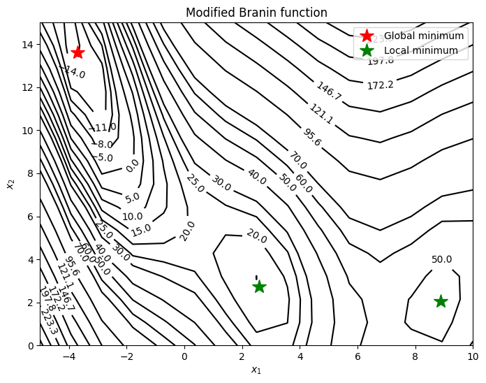
As can be seen from above plot, the function has multiple local minima and the goal is to find the global minimum using surrogate model and sequential sampling.