Lift#
This section is about estimating the lift model for the example airplane. At the conceptual phase, a simple lift model can be written as
where \(C_{L_\alpha}\) is the lift curve slope and \(\alpha_{L=0}\) is the angle of attack where the lift is zero. The \(\alpha_{L=0}\) is zero for an uncambered wing while it is non-zero for cambered wing. The \(\alpha_{L=0}\) can be approximated as the airfoil \(\alpha_{l=0}\) at mean chord location. Or \(\alpha_{L=0}\) can also be set to zero for simplifying the analysis. Note that this model is only for linear region of the lift curve.
Lift curve slope#
The most important parameter in this model is the lift curve slope. In the conceptual phase, it is important to estimate \(C_{L_\alpha}\). This is later used for setting wing incidence angle, computing drag polar, and in longitudinal stability analysis. The \(C_{L_\alpha}\) is estimated (in 1/radian) using a semi-empirical equation, written as
where A is the aspect ratio, \(\beta\) is the compressibility correction factor, given as
where \(M\) is the free-stream mach number. The \(\eta\) is the airfoil efficiency factor defined as
where \(C_{l_\alpha}\) is the airfoil lift curve slope in 1/radian. The \(\Lambda_{max,t/c}\) is the sweep angle at the chord fraction corresponding to maximum thickness. The \(S_{exposed}\) is defined as the wing reference area not covered by fuselage, while \(S_{ref}\) is the wing planform area (already computed). The \(F\) is the fuselage lift-factor given by
where \(d\) is the fuselage width and \(b\) is the wing span.
NOTE: The maximum value of the product of \(F\) and \(S_{exposed}/S_{ref}\) should not be more than 1
Below table summarizes various quantities for the example airplane that will be used for computing the lift-curve slope:
Parameter |
Value |
Source |
|---|---|---|
Aspect ratio, \(A\) |
8 |
from initial weight estimation |
Free stream mach number, \(M\) |
0.3 |
cruise condition, 200 knots at 8000 ft |
Airfoil efficiency, \(\eta\) |
1.0 |
assuming (Raymer 12.4.1) |
Wing span, \(b\) |
33 ft |
from wing planform section |
Fuselage width |
5 ft |
from fuselage sizing section |
Wing reference area, \(S_{ref}\) |
134 \(\text{ft}^2\) |
from constraint analysis |
Exposed reference area, \(S_{exposed}\) |
106 \(\text{ft}^2\) |
calculated using wing geometry and fuselage width |
Sweep at max camber, \(\Lambda_{max,t/c}\) |
\(\sim 0^{\circ}\) |
since max t/c at 30% and \(\Lambda_{25\%} = 0^{\circ}\) |
Zero-lift angle of attack, \(\alpha_{L=0}\) |
\(-1.0^{\circ}\) |
approximated from airfoil data |
Below code computes the lift curve slope at in clean configuration and cruise conditions:
# Variables
PI = 3.14159
A = 8
M = 0.3
b = 33 # ft
d = 5 # ft
S_ref = 134 # sq ft
S_exposed = 106 # sq ft

beta = (1 - M**2)**0.5
eta = 1.0
F = 1.07*(1 + d/b)**2

# Lift-curve slope - airplane
numerator = 2*PI*A*min(S_exposed*F/S_ref,0.98)
denominator = 2 + (4 + (A*beta/eta)**2)**0.5 # tan term is removed since tan(0) = 0

CLalpha = numerator / denominator

print(f"Lift-curve slope for airplane: {CLalpha:.2} 1/rad")
Lift-curve slope for airplane: 5.0 1/rad
Maximum \(C_L\) (clean)#
Along with lift-curve slope, it is important to compute the maximum \(C_L\) that the airplane can achieve in clean configuration (without the use of high-lift devices). It is very challenging to estimate maximum \(C_L\) even with wind tunnel experiments. In this sub-section, semi-empirical methods are used to get an estimate for maximum lift coefficient. As described in Raymer Section 12.4.5, following equation can be used for computing the maximum \(C_L\):
where \(C_{l_{max}}\) is the maximum \(C_l\) for the airfoil in similar flow conditions. The first term represents maximum \(C_L\) at Mach 0.2, while the second term is used as a correction factor for higher Mach number. Accordingly, angle of attack at maximum \(C_L\) can be computed as:
where \(\Delta \alpha_{C_{L_{max}}}\) is the change in \(\alpha\) due to the nonlinear affects near stall. Refer to Raymer Section 12.4.5 for further details.
Following table summarizes the required quantities for computing \(C_{L_{max}}\) and \(\alpha_{C_{L_{max}}}\):
Parameter |
Value |
Source |
|---|---|---|
\(C_{l_{max}}\) |
1.88 |
XFOIL analysis for NACA 23018 |
\(\alpha_{L=0}\) |
\(-1.0^{\circ}\) |
approximated from airfoil data |
\(C_{L_\alpha}\) |
5 \(\text{ rad}^{-1}\) |
calculated |
\(C_{L_{max}}/C_{l_{max}} \) |
0.9 |
Fig. 12.9, Raymer |
\(\Delta C_{L_{max}}\) |
-0.25 |
Fig. 12.10, Raymer |
\(\Delta \alpha_{C_{L_{max}}}\) |
\(2.5^{\circ}\) |
Fig. 12.11, Raymer |
Below code block computes maximum \(C_L\) and corresponding \(\alpha\) for the example airplane:
# Variables
Clmax = 1.88
alpha_zero_lift = -1.0
maxCl_ratio = 0.9
delta_CLmax = -0.25
detla_alpha_CLmax = 2.5

# maximum CL
CLmax = Clmax * maxCl_ratio + delta_CLmax

# alpha at max CL
alpha_CLmax = CLmax/CLalpha*180/PI + alpha_zero_lift + detla_alpha_CLmax

# Print
print(f"Maximum lift coefficient: {CLmax:.3}")
print(f"Alpha at maximum lift coefficient: {alpha_CLmax:.3} deg")
Maximum lift coefficient: 1.44
Alpha at maximum lift coefficient: 18.1 deg
NOTE: The \(C_{L_{max}}\) obtained above is very close to the value of 1.5 assumed in constraint analysis section
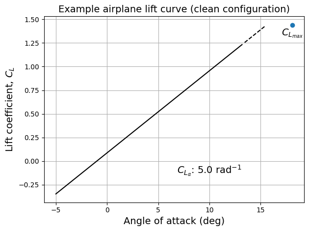
Lift curve plot#
Below code block plots lift curve, along with a point denoting \(C_{L_{max}}\) and \(\alpha_{C_{L_{max}}}\), for a range of \(\alpha\) values:
import numpy as np
import matplotlib.pyplot as plt

fs = 14 # fontsize
alpha = np.linspace(-5,20,100) * PI/180 # alpha values, rad
alpha_CLzero = -1.0 # assumed, deg

CL = CLalpha * (alpha - alpha_CLzero * PI/180)

# Splitting data based on linear and nonlinear region
CL_linear = CL[CL<=1.25]
alpha_linear = alpha[CL<=1.25]

CL_nonlinear = CL[np.logical_and(CL>1.25,CL<CLmax)]
alpha_nonlinear = alpha[np.logical_and(CL>1.25,CL<CLmax)]

fig, ax = plt.subplots()
ax.plot(alpha_linear*180/PI, CL_linear, "k-")
ax.plot(alpha_nonlinear*180/PI, CL_nonlinear, "k--")
ax.scatter(alpha_CLmax, CLmax)
ax.set_xlabel("Angle of attack (deg)", fontsize=fs)
ax.set_ylabel("Lift coefficient, $C_L$", fontsize=fs)
ax.set_title("Example airplane lift curve (clean configuration)", fontsize=fs)
ax.annotate(r"$C_{L_\alpha}$: " + f"{CLalpha:.2} " + r"$\text{rad}^{-1}$", (10,-0.1), fontsize=fs, ha="center", va="center")
ax.annotate("$C_{L_{max}}$", (18.1,1.35), fontsize=fs, ha="center", va="center")
ax.grid()
plt.tight_layout()
This concludes the lift section for the example airplane. Lift with high-lift devices will be covered later.