Matching process#
This section combines all the requirements and plots them on a single plot. The feasible region under all the constraints is also highlighted. An initial estimate of wing and power loading is also provided towards the end of this section.
Below code snippet imports required packages and creates a grid of \(W/S\) and \(W/P\) values for computing various constraints:
import numpy as np
import matplotlib.pyplot as plt
import matplotlib as mpl

# W/S and W/P values - sealevel at takeoff power
num_pts = 500
wing_loading = np.linspace(15, 50, num_pts) # lb/ft^2
power_loading = np.linspace(5, 20, num_pts) # lb/hp
X, Y = np.meshgrid(wing_loading, power_loading)
Takeoff distance#
Below code block computes takeoff distance requirement, refer here for further details.
s_tgr = 1500 # ft
sigma = 1 # since sealevel conditions
CL_max_to = 1.8

# coeff of quadratic eq
a = 0.009
b = 4.9
c = -s_tgr

# TOP solution
top_23 = (-b + np.sqrt(b**2 - 4*a*c)) / 2 / a # other solution will be negative

takeoff_req = X * Y / sigma / CL_max_to - top_23
Landing distance#
Below code snippet computes landing distance requirement, refer here for further details.
s_lgr = 1500 # ft
density_sea_level = 0.002387 # slugs/cu. ft
CL_max_L = 2.2 # assumed
wl_by_w_to = 0.975

# stall speed
v_sL = (s_lgr/0.265)**0.5 # in knots
v_sL = v_sL * 1.68781 # in ft/s

landing_req =  wl_by_w_to * X * 2 / density_sea_level / CL_max_L - v_sL**2
Climb Gradient#
Below code computes climb gradient requirement, refer here for further details. Note that only OEI scenario is included since it is the driving constraint among all the climb requirements.
# Variables
cgr = 0.015
sigma = 0.858 # 5000 ft
CL = 1.3
CD0 = 0.028 + 0.005
e = 0.81
A = 8
n_p = 0.8
wcr_by_wto = 0.975
p5000_by_pTO = 0.834

CD = CD0 + CL**2/np.pi/A/e
L_by_D = CL / CD
cgrp_oei = ( cgr + L_by_D**(-1) ) / CL**0.5

cgr_oei_req = Y * 2 / p5000_by_pTO * X**0.5 * wcr_by_wto**1.5 - 18.97 * n_p * sigma**0.5 / cgrp_oei
Cruise Speed#
Below code block computes cruise speed requirement, refer here for further details.
# Variables
ip = 1.4
sigma = 0.786
p8000_by_pTO = 0.758

cruise_speed_req = sigma * ip**3 * Y / p8000_by_pTO / 0.8 - X # 0.8 is for 80% power setting adjustment
Final plot#
Below code block plots all the requirements together and highlights the feasible region:
# Plotting
fs = 12 # fontsize
colors = ['r', 'b', 'g', 'k']

fig, ax = plt.subplots()

# Active constraint lines
cp = ax.contour(X, Y, takeoff_req, colors=colors[0], levels=[0])
mpl.rcParams['hatch.color'] = colors[0]
ax.contourf(X, Y, takeoff_req, levels=[0, 10], colors='none', hatches=['//'])

cp = ax.contour(X, Y, landing_req, colors=colors[1], levels=[0])
mpl.rcParams['hatch.color'] = colors[1]
ax.contourf(X, Y, landing_req, levels=[0, 200], colors='none', hatches=['//'])

cp = ax.contour(X, Y, cgr_oei_req, colors=colors[2], levels=[0])
mpl.rcParams['hatch.color'] = colors[2]
ax.contourf(X, Y, cgr_oei_req, levels=[0, 5], colors='none', hatches=['//'], alpha=0)

cp = ax.contour(X, Y, cruise_speed_req, colors=colors[3], levels=[0])
mpl.rcParams['hatch.color'] = colors[3]
ax.contourf(X, Y, cruise_speed_req, levels=[0, 2], colors='none', hatches=['\\\\'], alpha=0)

# Feasible region
feasbile_region = np.logical_and.reduce([takeoff_req <= 0, landing_req <= 0, cgr_oei_req <= 0, cruise_speed_req <= 0])
ax.contourf(wing_loading, power_loading, feasbile_region, colors="r", levels=[0.5,1], alpha=0.5)
ax.annotate("Feasible", (35,7), fontsize=14, va="center", ha="center")

# Annotation
ax.annotate("Takeoff", (30,15), ha="center", va="center", fontsize=fs)
ax.annotate("Landing", (46,17), ha="center", va="center", fontsize=fs)
ax.annotate("Climb OEI", (22,13), ha="center", va="center", fontsize=fs)
ax.annotate("Cruise speed", (20,7.5), ha="center", va="center", fontsize=fs)

# Design point
ax.scatter(40, 9.25, marker="*", s=100, label="Initial design point")

ax.legend(fontsize=fs-2, loc="upper center")
ax.set_xlabel("Wing Loading ($W/S$) [lbs/$ft^2$]", fontsize=fs)
ax.set_ylabel("Power Loading ($W/P$) [lbs/hp]", fontsize=fs)
ax.set_title("Matching process for the example airplane")
ax.tick_params(axis='both', labelsize=fs-2)
plt.tight_layout()
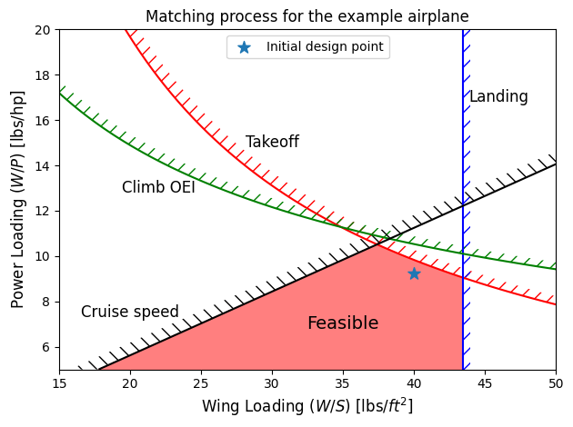
Based on the above plot, the initial estimates for \(W/S\) and \(W/P\) are selected as 40 lbs/\(\text{ft}^2\) and 9.25 lbs/hp, respectively. Refer to the lecture notes for more details about selecting initial design point.