Landing

This section performs landing analysis for the example airplane using the method described in Raymer Section 17.9. Similar to takeoff, the landing analysis is divided into four parts - approach distance, flare distance, free roll, and braking distance. Refer to Figure 17.19 in Raymer for a visual depiction of these phases. Hence, total landing distance \(S_l\) is defined as

\[ S_l = S_a + S_f + S_{fr} + S_b \]

where \(S_{a}\) is the approach distance, \(S_f\) is the flare distance, \(S_{fr}\) is the horizontal distance covered during free roll, and \(S_b\) is the braking distance. Note that the total landing ground roll distance \(S_{gr}\) will be summation of \(S_{fr}\) and \(S_b\). The following sub-sections compute the distance traveled in each phase.

Approach

The approach phase starts from obstacle clearance height \(h_{obs}\) above the runway and continues till the start of flare. The horizontal distance covered during approach can be computed as (equation 17.112, Raymer)

\[ S_a = \frac{h_{obs} - h_f}{\tan \gamma_a}, \]

where \(h_f\) is the flare height. The approach anlge \(\gamma_a\) is usually \(3^{\circ}\) for a passenger airplane. Note that maintaining \(\gamma_a\) of \(3^{\circ}\) might require more than idle thrust. The \(h_{obs}\) is 50 ft for the example airplane (FAR Part 23). The \(h_f\) is computed using

\[ h_f = R(1 - \cos \gamma_a), \]

where \(R\) is the radius of the circular arc that approximates the flare phase. The \(R\) is computed using

\[ R = \frac{V_f^2}{0.2g}, \]

where \(V_f\) is the average speed during flare and is usually 1.23 times the stall speed. Note that the stall speed is computed in landing configuration. The landing weight is set to 95% of the maximum takeoff weight, while the \(C_{L_{max_L}}\) is 2.2.

Below code block computes appraoch distance \(S_a\):

import numpy as np

# Parameters
W_loading = 0.95 * 5374 # lbs
Sref = 134 # sq ft
rho = 0.00237717 # slugs/cu ft, sea-level
CLmax_L = 2.2
g = 32.2 # ft/s^2
gamma_approach = 3 # deg
hobs = 50 # ft

Vf = 1.23 * ( W_loading/Sref * 2 / rho / CLmax_L)**0.5

Va = 1.3 * ( W_loading/Sref * 2 / rho / CLmax_L)**0.5

print(f"Approach speed: {Va:.0f} ft/s")
print(f"Average flare speed: {Vf:.0f} ft/s")

R = Vf**2 / 0.2 / g

hf = R * (1 - np.cos(np.radians(gamma_approach)))

print(f"Flare height: {hf:.0f} ft")

Sa = (hobs - hf) / np.tan(np.radians(gamma_approach))

print(f"Approach distance: {Sa:.0f} ft")

Approach speed: 157 ft/s
Average flare speed: 148 ft/s
Flare height: 5 ft
Approach distance: 865 ft

Flare

During flare, airplane transitions from stable decent angle by pitching the nose up and decelerating from approach speed \(V_a\) to touchdown speed \(V_{td}\) (usually 1.15 times stall speed). Hence, the average speed during flare is 1.23 times stall speed. The horizontal distance covered during flare is computed using

\[ S_f = R \sin \gamma_a. \]

Below code block computes the flare distance:

Sf = R * np.sin(np.radians(gamma_approach))

print(f"Flare distance: {Sf:.0f} ft")

Flare distance: 179 ft

Free roll

The distance covered during free roll \(S_{fr}\) depends on how quickly pilots apply brake after touchdown. The \(S_{fr}\) can be estimated using the touchdown speed and time for free roll, assuming that there is no deceleration in this phase. It is assumed that it takes about 1 seccond before brakes are applied. Below code block computes \(S_{fr}\):

Vtd = Vf / 1.23 * 1.15 # ft/s
t_free_roll = 1 # sec
Sfr = Vtd * t_free_roll # ft

print(f"Touchdown speed: {Vtd:.0f} ft/s")

print(f"Distance travelled during free roll: {Sfr:.0f} ft")

Touchdown speed: 139 ft/s
Distance travelled during free roll: 139 ft

Braking distance

The braking distance \(S_b\) can be calculated similar to ground roll in takeoff analysis. Using equation 17.102 in Raymer, the \(S_b\) can be computed as

\[ S_b = \frac{1}{2gK_a} \ln \bigg( \frac{K_t}{K_t + K_aV_{td}^2} \bigg), \]

where \(K_a\) and \(K_t\) are defined as (equation 17.103 and 17.104, Raymer)

\[ K_t = - \mu \quad \text{and} \quad K_a = \frac{\rho}{2(W/S)} (\mu C_L - C_{D_0} - KC_{L}^2). \]

The \(\mu\) is the rolling resistance coefficient with brakes applied, \(C_L\) is the lift coefficient based on the angle of attack experienced by the plane on ground, and \(C_{D_0}\) is the parasitic drag coefficient in landing configuration. Note that, in the above formula, \(K_t\) is for zero thrust only.

Below code block computes braking distance and total ground roll:

A = 8
e = 0.81 - 0.1 # in landing conditions
mu = 0.5 # Raymer Table 17.1, with brakes
CD0 = 0.03363 + 0.048074 # landing conditions
CL = 0.9 # Landing lift curve with wing incidence of 2 deg

# K in drag model
K = 1/np.pi/A/e
h = 4 # ft, height of wing above ground
b = 33 # ft, wing span
Keff = K * ( 33 * (h/b)**1.5 / ( 1 + 33 * (h/b)**1.5 ) ) # eq 12.60, Raymer

# braking distance distance
KT = - mu # zero thrust
KA = rho / 2 / W_loading / Sref * (mu*CL - CD0 - Keff*CL**2)
Sb = np.log( KT / (KT + KA*Vtd**2) ) / 2 / g / KA

print(f"Braking distance: {Sb:.0f} ft")

Braking distance: 598 ft

Below code block computes total ground roll and total landing distance:

Sgr = Sb + Sfr

print(f"Total ground roll distance: {Sgr:.0f} ft")

Sl = Sa + Sf + Sfr + Sb

print(f"Total landing distance: {Sl:.0f} ft")

Total ground roll distance: 737 ft
Total landing distance: 1781 ft

Note that the total ground roll distance is less than the required limit of 1500 ft. Below image summarizes the final result from the landing analysis:

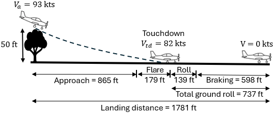
This concludes the landing analysis, next section is about climb analysis.