Problem Formulation#
This section provides implementation for concepts related to optimization problem formulation. Following block of code imports required packages.
import matplotlib.pyplot as plt
import numpy as np
import matplotlib

matplotlib.rcParams['contour.negative_linestyle'] = 'solid'
Example 1#
Consider the following optimization problem:
Question 1: Transcribe the problem into the standard design optimization problem.
Answer:
There is one constraint and three bounds on the design variables.
Question 2: Plot the objective contours and constraints.
Answer: Following block of code defines a python function which returns function, constraint, and bound values at given \(x_1\) and \(x_2\).
def function_1(x1, x2):
"""
Function to calculate the value of function, constraints and bounds
at given x values.
"""
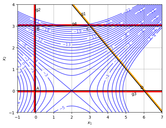
f = x1**2 - 2*x2**2 - 4*x1
g1 = x1 + x2 - 6
g2 = -x1
g3 = -x2
g4 = x2 - 3
return f, g1, g2, g3, g4
Following block of code uses the above defined function for plotting.
# Defining x1 and x2 values
x1 = np.linspace(-1,7,100)
x2 = np.linspace(-1,4,100)

# Creating a mesh at which values and
# gradient will be evaluated and plotted
X1, X2 = np.meshgrid(x1, x2)

# Evaluating the value and gradient
Z, g1, g2, g3, g4 = function_1(X1,X2)

# Plotting the graph
fig, ax = plt.subplots()

# Function contour
CS = ax.contour(X1, X2, Z, levels=np.arange(-22, 5, 1), colors='b', alpha=0.7)
ax.clabel(CS, inline=1, fontsize=10)

# Constraint 1
ax.contour(X1, X2, g1, levels=[0], colors='k')
ax.contourf(X1, X2, g1, levels=[0.01, 0.1], colors='orange')
ax.annotate('g1', xy=(2.5, 3.5))

# Constraint 2
ax.contour(X1, X2, g2, levels=[0], colors='k')
ax.contourf(X1, X2, g2, levels=[0.01, 0.1], colors='red')
ax.annotate('g2', xy=(0.0, 3.7))

# Cosntraint 3
ax.contour(X1, X2, g3, levels=[0], colors='k')
ax.contourf(X1, X2, g3, levels=[0.01, 0.07], colors='red')
ax.annotate('g3', xy=(5.3, -0.2))

# Cosntraint 4
ax.contour(X1, X2, g4, levels=[0], colors='k')
ax.contourf(X1, X2, g4, levels=[0.01, 0.07], colors='red')
ax.annotate('g4', xy=(2, 3.05))

# Few annotations
ax.annotate('A', xy=(0.05, 0.05))
ax.annotate('B', xy=(0.05, 2.8))
ax.annotate('C', xy=(2.8, 2.8))
ax.annotate('D', xy=(5.8, 0.1))

ax.set_xlabel("$x_1$")
ax.set_ylabel("$x_2$")
ax.grid()

plt.show()
Legend for the above plot:
Blue lines: Contour lines for function values. Black lines: Line where constraint/bound is active. Orange/Red thick lines: Shows infeasible side of the constraint/bound.
Question 3: Identify the feasible region, optimum solution, and the active constraint/bound(s).
Answer: Quadrilateral ABCDA is the feasible region. Optimum solution: \(x_1^* = 2\), \(x_2^* = 3\), \(f(2,3) = -22\), Active constraint/bound: \(b_1\). This shows that it is not necessary to have an optimum point in a corner.
Example 2#
Question 1: Plot the following objective function, constraints, and bounds in the x – y plane:
There are two constraints and two bounds on the design variables.
Answer: Following block of code defines a python function which returns function, constraint, and bound values at given x and y.
def function_2(x, y):
"""
Function to calculate the value of function at given x values.
"""
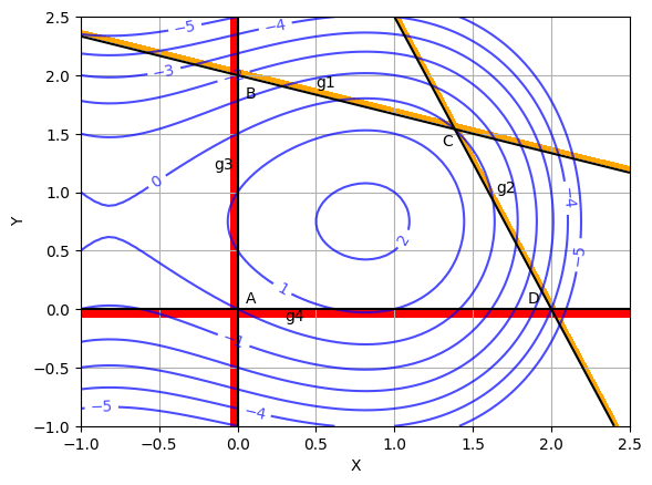
f = 2*x + 3*y - x**3 - 2*y**2
g1 = x + 3*y - 6
g2 = 5*x + 2*y - 10
g3 = -x
g4 = -y
return f, g1, g2, g3, g4
Following block of code uses above defined function for plotting.
# Defining x and y values
x = np.linspace(-1,2.5,80)
y = np.linspace(-1,2.5,80)

# Creating a mesh at which values and
# gradient will be evaluated and plotted
X, Y = np.meshgrid(x, y)

# Evaluating the value and gradient
Z, g1, g2, g3, g4 = function_2(X,Y)

# Plotting the graph
fig, ax = plt.subplots()

# Function contour
CS = ax.contour(X, Y, Z, levels=np.arange(-5, 5, 1), colors='b', alpha=0.7)
ax.clabel(CS, inline=1, fontsize=10)

# Constraint 1
ax.contour(X, Y, g1, levels=[0], colors='k')
ax.contourf(X, Y, g1, levels=[0.05, 0.15], colors='orange')
ax.annotate('g1', xy=(0.5, 1.9))

# Constraint 2
ax.contour(X, Y, g2, levels=[0], colors='k')
ax.contourf(X, Y, g2, levels=[0.05, 0.15], colors='orange')
ax.annotate('g2', xy=(1.65,1.0))

# Cosntraint 3
ax.contour(X, Y, g3, levels=[0], colors='k')
ax.contourf(X, Y, g3, levels=[0.001, 0.05], colors='red')
ax.annotate('g3', xy=(-0.15, 1.2))

# Cosntraint 4
ax.contour(X, Y, g4, levels=[0], colors='k')
ax.contourf(X, Y, g4, levels=[0.001, 0.07], colors='red')
ax.annotate('g4', xy=(0.3, -0.1))

# Few annotations
ax.annotate('A', xy=(0.05, 0.05))
ax.annotate('B', xy=(0.05, 1.8))
ax.annotate('C', xy=(1.3, 1.4))
ax.annotate('D', xy=(1.85, 0.05))

ax.set_xlabel("X")
ax.set_ylabel("Y")
ax.grid()

plt.show()
Legend for the above plot:
Blue lines: Contour lines for function values. Black lines: Line where constraint/bound is active. Orange/Red thick lines: Shows infeasible side of constraint/bound.
Question 2: Identify the feasible region. By visual inspection, determine minimum and maximum points for objective function. For each of those points, give objective function value, active constraints/bounds (if any).
Answer: Quadrilateral ABCDA is the feasible region. Since function value increases as you move inwards from boundary of feasible region, four corners will be minimum.
Local minimum: \(A(0,0)\) with \(f(0,0) = 0\). Active constraints/bounds: \(b_1\) and \(b_2\) Local minimum: \(B(0,2)\) with \(f(0,2) = -2\). Active constraints/bounds: \(g_1\) and \(b_1\) Local minimum: \(C(1.39,1.54)\) with \(f(1.39,1.54) = 0\). Active constraints/bounds: \(g_1\) and \(g_2\) Local minimum: \(D(2,0)\) with \(f(2,0) = -4\). Active constraints/bounds: \(g_2\) and \(b_2\)
Global minimum: \(D(2,0)\) with \(f(2,0) = -4\). Active constraints/bounds: \(g_2\) and \(g_4\)
Global maximum: \(E(0.82,0.75)\) with \(f(0.82,0.75) = 2.21\). Active constraints/bounds: None