Probability of Improvement

This section describes another approach for performing balanced exploration and exploitation. The next infill point is obtained by maximizing the probability of improvement (PI) given as

\[ PI(x) = P(\hat{f}(x) \leq f^*) = \Phi\left(\frac{f^* - \hat{f}(x)}{ \hat{\sigma}(x)}\right) \]

where \(\Phi\) is the cumulative distribution function of the standard normal distribution, \(f^*\) is the best observed value, and \(\hat{f}(x)\) and \(\hat{\sigma}(x)\) are the prediction and standard deviation from surrogate model at \(x\), respectively. The PI function is a measure of the probability that the improvement of surrogate model at \(x\) over the best observed value is greater than zero.

Below code imports required packages, defines modified branin function, and creates plotting data:

# Imports
import numpy as np
from smt.surrogate_models import KRG
from smt.sampling_methods import LHS, FullFactorial
import matplotlib.pyplot as plt
from pymoo.core.problem import Problem
from pymoo.algorithms.soo.nonconvex.de import DE
from pymoo.optimize import minimize
from pymoo.config import Config
Config.warnings['not_compiled'] = False
from scipy.stats import norm as normal

def modified_branin(x):

    dim = x.ndim

    if dim == 1:
        x = x.reshape(1, -1)

    x1 = x[:,0]
    x2 = x[:,1]

    a = 1.
    b = 5.1 / (4.*np.pi**2)
    c = 5. / np.pi
    r = 6.
    s = 10.
    t = 1. / (8.*np.pi)

    y = a * (x2 - b*x1**2 + c*x1 - r)**2 + s*(1-t)*np.cos(x1) + s + 5*x1

    if dim == 1:
        y = y.reshape(-1)

    return y

# Bounds
lb = np.array([-5, 0])
ub = np.array([10, 15])

# Plotting data
sampler = FullFactorial(xlimits=np.array( [[lb[0], ub[0]], [lb[1], ub[1]]] )) 
num_plot = 400
xplot = sampler(num_plot)
yplot = modified_branin(xplot)

Differential evolution (DE) from pymoo is used for minimizing the surrogate model. Below code defines problem class and initializes DE. Note how problem class is using both prediction and uncertainty together.

# Problem class
class PI(Problem):

    def __init__(self, sm, ymin):
        super().__init__(n_var=2, n_obj=1, n_constr=0, xl=lb, xu=ub)

        self.sm = sm # store the surrogate model
        self.ymin = ymin

    def _evaluate(self, x, out, *args, **kwargs):

        numerator = self.ymin - self.sm.predict_values(x)
        denominator = np.sqrt( self.sm.predict_variances(x) ) # sigma
        
        # Computing probability of improvement
        out["F"] = - normal.cdf(numerator/denominator) # PI

# Optimization algorithm
algorithm = DE(pop_size=100, CR=0.8, dither="vector")

Below block of code creates 5 training points and performs sequential sampling using PI. The maximum number of iterations is set to 20 and a convergence criterion is defined based on maximum value of PI obtained in each iteration.

sampler = LHS( xlimits=np.array( [[lb[0], ub[0]], [lb[1], ub[1]]] ), criterion='ese')

# Training data
num_train = 5
xtrain = sampler(num_train)
ytrain = modified_branin(xtrain)

# Variables
itr = 0
max_itr = 20
tol = 1e-2
max_PI = [1]
ybest = []
bounds = [(lb[0], ub[0]), (lb[1], ub[1])]
corr = 'squar_exp'
fs = 12

# Sequential sampling Loop
while itr < max_itr and tol < max_PI[-1]:
    
    print("\nIteration {}".format(itr + 1))

    # Initializing the kriging model
    sm = KRG(theta0=[1e-2], corr=corr, theta_bounds=[1e-6, 1e2], print_global=False)

    # Setting the training values
    sm.set_training_values(xtrain, ytrain)
    
    # Creating surrogate model
    sm.train()

    # Find the best observed sample
    ybest.append(np.min(ytrain))

    # Find the minimum of surrogate model
    result = minimize(PI(sm, ybest[-1]), algorithm, verbose=False)
    
    # Computing true function value at infill point
    y_infill = modified_branin(result.X.reshape(1,-1))
    
    # Storing variables
    if itr == 0:
        max_PI[0] = -result.F[0]
        xbest = xtrain[np.argmin(ytrain)].reshape(1,-1)
    else:
        max_PI.append(-result.F[0])
        xbest = np.vstack((xbest, xtrain[np.argmin(ytrain)]))

    print("Maximum PI: {}".format(max_PI[-1]))
    print("Best observed value: {}".format(ybest[-1]))
    
    # Appending the the new point to the current data set
    xtrain = np.vstack(( xtrain, result.X.reshape(1,-1) ))
    ytrain = np.append( ytrain, y_infill )
    
    itr = itr + 1 # Increasing the iteration number

# Printing the final results
print("\nBest obtained point:")
print("x*: {}".format(xbest[-1]))
print("f*: {}".format(ybest[-1]))

Iteration 1
Maximum PI: 0.5307276253640137
Best observed value: -8.969989311850687

Iteration 2
Maximum PI: 1.0
Best observed value: -8.969989311850687

Iteration 3
Maximum PI: 1.0
Best observed value: -10.539622928100016

Iteration 4
Maximum PI: 1.0
Best observed value: -10.548222713569086

Iteration 5
Maximum PI: 1.0
Best observed value: -10.811096859780191

Iteration 6
Maximum PI: 1.0
Best observed value: -10.846424691094906

Iteration 7
Maximum PI: 0.9999999823974798
Best observed value: -10.846586669519857

Iteration 8
Maximum PI: 1.0
Best observed value: -11.370843631821975

Iteration 9
Maximum PI: 1.0
Best observed value: -12.62827813750655

Iteration 10
Maximum PI: 1.0
Best observed value: -12.930375341448068

Iteration 11
Maximum PI: 1.0
Best observed value: -12.934593556882668

Iteration 12
Maximum PI: 1.0
Best observed value: -13.879940903713123

Iteration 13
Maximum PI: 1.0
Best observed value: -15.106508885431069

Iteration 14
Maximum PI: 1.0
Best observed value: -16.00839750811641

Iteration 15
Maximum PI: 0.04716145526030488
Best observed value: -16.30471397961604

Iteration 16
Maximum PI: 0.10552741488639861
Best observed value: -16.30471397961604

Iteration 17
Maximum PI: 1.0
Best observed value: -16.30471397961604

Iteration 18
Maximum PI: 0.0007970175519111094
Best observed value: -16.496788707181345

Best obtained point:
x*: [-3.8761853  14.01060158]
f*: -16.496788707181345

Below code plots the convergence of best observed value and PI.

####################################### Plotting convergence history

fig, ax = plt.subplots(1, 2, figsize=(14,6))
ax[0].plot(np.arange(itr) + 1, xbest[:,0], c="black", label='$x_1^*$', marker=".")
ax[0].plot(np.arange(itr) + 1, xbest[:,1], c="green", label='$x_2^*$', marker=".")
ax[0].plot(np.arange(itr) + 1, ybest, c="blue", label='$f^*$', marker=".")
ax[0].set_xlabel("Iterations", fontsize=14)
ax[0].set_ylabel("Best observed $f^*$ and ($x_1^*$, $x_2^*$)", fontsize=14)
ax[0].legend()
ax[0].set_xlim(left=1, right=itr-1)
ax[0].grid()

ax[1].plot(np.arange(itr) + 1, max_PI, c="red", marker=".")
ax[1].plot(np.arange(itr) + 1, [tol]*(itr), c="black", linestyle="--", label="Tolerance")
ax[1].set_xlabel("Iterations", fontsize=14)
ax[1].set_ylabel("Maximum PI", fontsize=14)
ax[1].set_xlim(left=1, right=itr)
ax[1].grid()
ax[1].legend()
ax[1].set_yscale("log")

fig.suptitle("Probability of Improvement", fontsize=15)

Text(0.5, 0.98, 'Probability of Improvement')

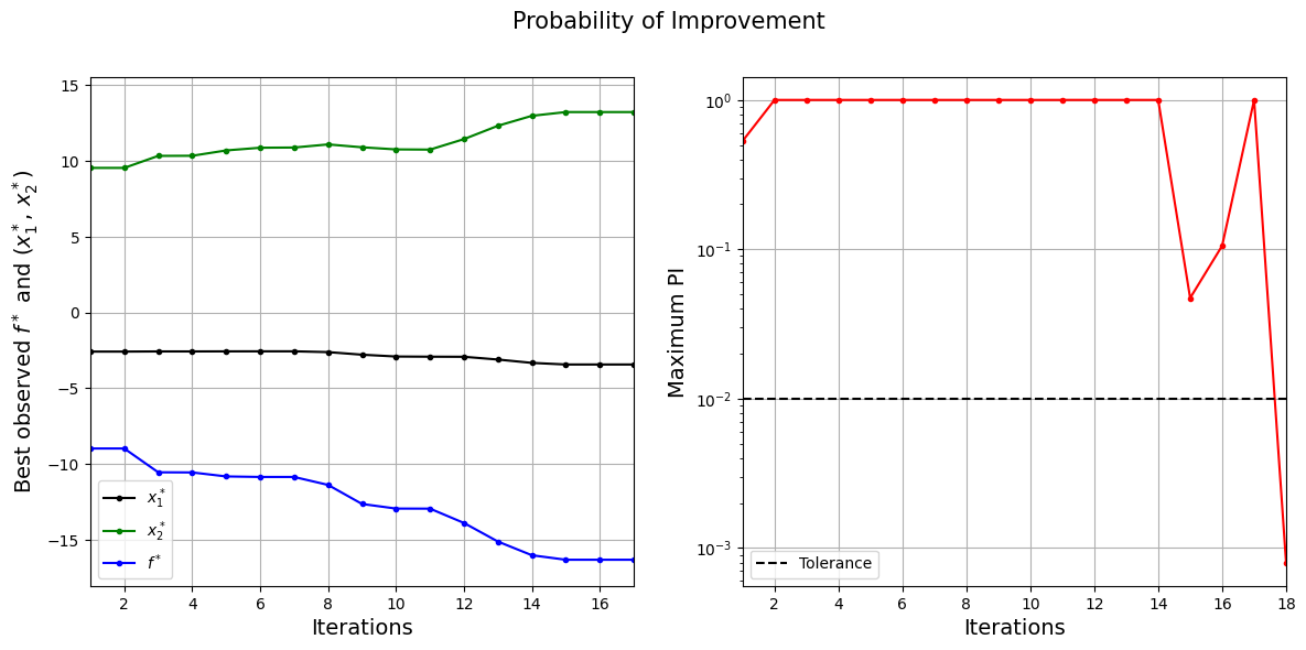
The figure on left shows the history of best observed \(y\) value and corresponding \(x\) values, and figure on right shows the convergence of PI. At the start, the PI is high since the possibility to find a better point is high. As the iterations progress, the best observed value reaches the global minimum and the PI decreases since there is less possibility to find a better point.

Below code plots the infill points.

####################################### Plotting initial samples and infills

# Reshaping into grid
reshape_size = int(np.sqrt(num_plot))
X = xplot[:,0].reshape(reshape_size, reshape_size)
Y = xplot[:,1].reshape(reshape_size, reshape_size)
Z = yplot.reshape(reshape_size, reshape_size)

# Level
levels = np.linspace(-17, -5, 5)
levels = np.concatenate((levels, np.linspace(0, 30, 7)))
levels = np.concatenate((levels, np.linspace(35, 60, 5)))
levels = np.concatenate((levels, np.linspace(70, 300, 12)))

fig, ax = plt.subplots(figsize=(8,6))
CS=ax.contour(X, Y, Z, levels=levels, colors='k', linestyles='solid', alpha=0.5, zorder=-10)
ax.clabel(CS, inline=1, fontsize=8)
ax.scatter(xtrain[0:num_train,0], xtrain[0:num_train,1], c="red", label='Initial samples')
ax.scatter(xtrain[num_train:,0], xtrain[num_train:,1], c="black", label='Infills')
ax.plot(-3.689, 13.630, 'g*', markersize=15, label="Global minimum")
ax.plot(xbest[-1,0], xbest[-1,1], 'bo', label="Obtained minimum")
ax.legend()
ax.set_xlabel("$x_1$", fontsize=14)
ax.set_ylabel("$x_2$", fontsize=14)
ax.set_title("Modified Branin function", fontsize=15)

Text(0.5, 1.0, 'Modified Branin function')

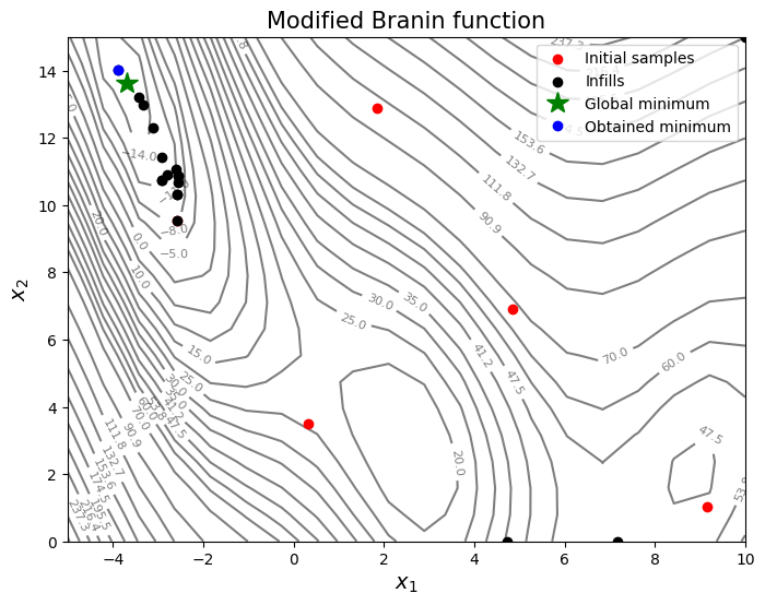
Based on the infills, PI seems to be slightly more biased towards adding points close to the minimum values in the dataset - less exploration and more exploitation - and there is no way to control that through the criteria itself. As discussed in the lecture, PI provides only a probability value and doesn’t quantify the amount of improvement.

NOTE: Due to randomness in differential evolution, results may vary slightly between runs. So, it is recommended to run the code multiple times to see average behavior.

Final result:

Parameter	True minimum	Obtained minimum
\(x_1^*\)	-3.689	-3.876
\(x_2^*\)	13.630	14.011
\(f(x_1^*, x_2^*)\)	-16.644	-16.497