Uniform Distribution

A continuous random variable \(X\) is said to have a uniform distribution on the interval \([A, B]\) if the pdf of \(X\) is:

\[\begin{split} f(x;A,B) = \begin{cases} \frac{1}{B-A} & A \leq X \leq B \\ 0 & \text{otherwise} \end{cases} \end{split}\]

This distribution essentially denotes that any value is equally likely between \(A\) and \(B\). The statement that \(X\) has a uniform distribution on \([A, B]\) will be denoted by \(X \sim\) Unif \([A, B]\). Now, we will look at an example for this distribution.

Example: Suppose the reaction temperature \(X\) (in \(^{\circ}\)C) in a chemical process has a uniform distribution with \(A = -10\) and \(B = 20\). Thus, pdf of \(X\) will be:

\[\begin{split} f(x;A,B) = \begin{cases} \frac{1}{30} & -10 \leq X \leq 20 \\ 0 & \text{otherwise} \end{cases} \end{split}\]

Now, let’s use uniform object within scipy.stats module to answer various questions related to this example. By default, uniform object will be in standard form i.e. \(A = 0\) and \(B = 1\). So, we need to mention loc (which is A) and scale (which is B - A). Reading the documentation for uniform distribution implemented in scipy will help.

NOTE: You need to install seaborn before proceeding further. Activate the environment you created for this class in the anaconda prompt and install seaborn using pip install seaborn.

Following block imports all the required packages:

from scipy.stats import uniform
import matplotlib.pyplot as plt
import numpy as np
import seaborn as sns

Question: Compute mean, variance and standard deviation of this distribution.

Answer: Once uniform object is imported, you can access various function related to the distribution. To compute the quantities, function within uniform object is used as shown in following block.

# Defining starting point and range of uniform distribution
# loc = A
# scale = B - A
A = -10
B = 20
loc = A
scale = B - A

# Creating uniform distribution object with fixed location and scale parameters
rv = uniform(loc=loc, scale=scale)

# Compute mean of the distribution
print("Mean for this distribution: {}".format(rv.mean()))

# Compute variance of the distribution
print("Variance for this distribution: {}".format(rv.var()))

# Compute std-dev of the distribution
print("Standard deviation for this distribution: {}".format(rv.std()))

Mean for this distribution: 5.0
Variance for this distribution: 75.0
Standard deviation for this distribution: 8.660254037844387

Question: Compute \(P(X < 10)\).

Answer: Here, \(P(X < 10) = P(X \leq 10) = F(10)\). So, we have to compute cdf for uniform distribution at \(10\). You can do this as shown in following block:

# P(X<10)
rv.cdf(10)

0.6666666666666666

Question: Compute \(P(-5 < X < 5)\):

Answer: Here, \(P(-5 < X < 5) = P(-5 \leq X \leq 5) = F(5) - F(-5)\). So, we have to compute cdf for uniform distribution at \(5\) and \(-5\). You can do this calculating as shown in following block:

# P(-5 < X < 5)
rv.cdf(5) - rv.cdf(-5)

0.33333333333333337

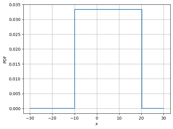
Question: Plot cdf and pdf of the distribution.

Answer: We can use the rv object created in previous block and compute value of pdf and cdf at a bunch of x values. Then, use matplotlib to plot them. Code in the following block executes this task.

# Creating array of x values at which pdf and cdf will be computed while plotting
x = np.linspace(-30, 30, 100)

# Plotting PDF
fig, ax = plt.subplots()
ax.step(x, rv.pdf(x), where='post')
ax.set_xlabel("$x$")
ax.set_ylabel("PDF")
ax.grid()
plt.show()

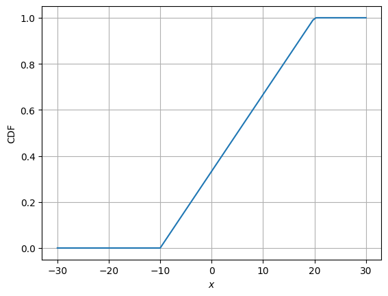
# Plotting CDF
fig, ax = plt.subplots()
ax.plot(x, rv.cdf(x))
ax.set_xlabel("$x$")
ax.set_ylabel("CDF")
ax.grid()
plt.show()

Now, we will look into frequency interpretation of probability. You can read more about it here. Below code plots the distribution of samples drawn from uniform distribution. Number of samples initially is set to 10 and with every iteration it increases by an order of magnitude.

# Some settings
initial_samples = 10
iter = 6

for i in range(iter):
    # Number of samples
    samples = initial_samples*10**(i)

    # Generate samples from the distribution
    data = rv.rvs(size=samples)

    # Plotting using seaborn
    fig, ax = plt.subplots()
    plot = sns.histplot(data, stat="density", ax=ax)
    ax.set_xlabel("x")
    ax.set_xlim([-20, 40])

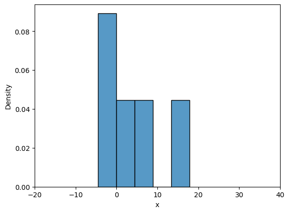
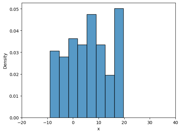
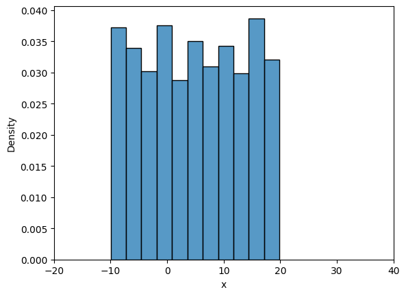
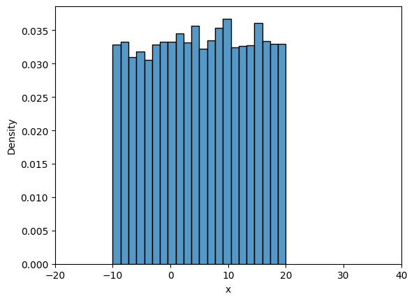
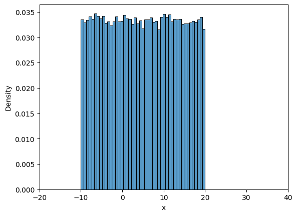
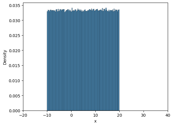
Note that all the samples are between \(A\) and \(B\), and as the number of samples increase the density value approaches \(1/30\) which is the theortical density value. You can play around with the value of iter, initial_samples, \(A\), \(B\) and see how distribution changes.