Expected Improvement

This section demonstrates Expected Improvement (EI) which is the most widely used criteria for performing balanced exploration and exploitation. The next infill point is obtained by maximizing EI which is written as

\[\begin{split} EI(x) = \begin{cases} [f^* - \hat{f}(x)] \cdot \Phi(\mathrm{Z}) + \hat{\sigma}(x) \cdot \phi(\textrm{Z}) & \text{if } \hat{\sigma}(x) > 0 \\ 0 & \text{if } \hat{\sigma}(x) = 0 \end{cases} \end{split}\]

where \(\Phi\) and \(\phi\) are cumulative distribution and probability density function of the standard normal distribution, \(f^*\) is the best observed value, and \(\hat{f}(x)\) and \(\hat{\sigma}(x)\) are the prediction and standard deviation from surrogate model at \(x\), respectively. \(\textrm{Z}\) is a standard normal variable computed as

\[ \textrm{Z} = \frac{f^* - \hat{f}(x)}{\hat{\sigma}(x)} \]

The EI is a measure of the expected improvement of surrogate model at \(x\) over the best observed value. The first term in EI represents exploitation and the second term represents exploration.

Below code imports required packages, defines modified branin function, and creates plotting data:

# Imports
import numpy as np
from smt.surrogate_models import KRG
from smt.sampling_methods import LHS, FullFactorial
import matplotlib.pyplot as plt
from pymoo.core.problem import Problem
from pymoo.algorithms.soo.nonconvex.de import DE
from pymoo.optimize import minimize
from pymoo.config import Config
Config.warnings['not_compiled'] = False
from scipy.stats import norm as normal

def modified_branin(x):

    dim = x.ndim

    if dim == 1:
        x = x.reshape(1, -1)

    x1 = x[:,0]
    x2 = x[:,1]

    a = 1.
    b = 5.1 / (4.*np.pi**2)
    c = 5. / np.pi
    r = 6.
    s = 10.
    t = 1. / (8.*np.pi)

    y = a * (x2 - b*x1**2 + c*x1 - r)**2 + s*(1-t)*np.cos(x1) + s + 5*x1

    if dim == 1:
        y = y.reshape(-1)

    return y

# Bounds
lb = np.array([-5, 0])
ub = np.array([10, 15])

# Plotting data
sampler = FullFactorial(xlimits=np.array( [[lb[0], ub[0]], [lb[1], ub[1]]] )) 
num_plot = 400
xplot = sampler(num_plot)
yplot = modified_branin(xplot)

Differential evolution (DE) from pymoo is used for maximizing EI. Below code defines problem class and initializes DE. Note how problem class is computing EI.

# Problem class
class EI(Problem):

    def __init__(self, sm, ymin):
        super().__init__(n_var=2, n_obj=1, n_constr=0, xl=lb, xu=ub)

        self.sm = sm # store the surrogate model
        self.ymin = ymin

    def _evaluate(self, x, out, *args, **kwargs):

        # Standard normal
        numerator = self.ymin - self.sm.predict_values(x)
        denominator = np.sqrt( self.sm.predict_variances(x) )
        z = numerator / denominator
        
        # Computing expected improvement
        # Negative sign because we want to maximize EI
        out["F"] = - ( numerator * normal.cdf(z) + denominator * normal.pdf(z) )

# Optimization algorithm
algorithm = DE(pop_size=100, CR=0.8, dither="vector")

Below block of code creates 5 training points and performs sequential sampling process using EI. The maximum number of iterations is set to 20 and a convergence criterion is defined based on maximum value of EI obtained in each iteration.

sampler = LHS( xlimits=np.array( [[lb[0], ub[0]], [lb[1], ub[1]]] ), criterion='ese')

# Training data
num_train = 5
xtrain = sampler(num_train)
ytrain = modified_branin(xtrain)

# Variables
itr = 0
max_itr = 20
tol = 1e-3
max_EI = [1]
ybest = []
bounds = [(lb[0], ub[0]), (lb[1], ub[1])]
corr = 'squar_exp'
fs = 12

# Sequential sampling Loop
while itr < max_itr and tol < max_EI[-1]:
    
    print("\nIteration {}".format(itr + 1))

    # Initializing the kriging model
    sm = KRG(theta0=[1e-2], corr=corr, theta_bounds=[1e-6, 1e2], print_global=False)

    # Setting the training values
    sm.set_training_values(xtrain, ytrain)
    
    # Creating surrogate model
    sm.train()

    # Find the best observed sample
    ybest.append(np.min(ytrain))

    # Find the minimum of surrogate model
    result = minimize(EI(sm, ybest[-1]), algorithm, verbose=False)
    
    # Computing true function value at infill point
    y_infill = modified_branin(result.X.reshape(1,-1))

    # Storing variables
    if itr == 0:
        max_EI[0] = -result.F[0]
        xbest = xtrain[np.argmin(ytrain)].reshape(1,-1)
    else:
        max_EI.append(-result.F[0])
        xbest = np.vstack((xbest, xtrain[np.argmin(ytrain)]))

    print("Maximum EI: {}".format(max_EI[-1]))
    print("Best observed value: {}".format(ybest[-1]))
    
    # Appending the the new point to the current data set
    xtrain = np.vstack(( xtrain, result.X.reshape(1,-1) ))
    ytrain = np.append( ytrain, y_infill )
    
    itr = itr + 1 # Increasing the iteration number

# Printing the final results
print("\nBest obtained point:")
print("x*: {}".format(xbest[-1]))
print("f*: {}".format(ybest[-1]))

Iteration 1
Maximum EI: 7.987087326181626
Best observed value: -5.917796596335452

Iteration 2
Maximum EI: 2.265360619429096
Best observed value: -5.917796596335452

Iteration 3
Maximum EI: 11.745641166366296
Best observed value: -5.917796596335452

Iteration 4
Maximum EI: 10.738012145118145
Best observed value: -5.917796596335452

Iteration 5
Maximum EI: 9.39191947660995
Best observed value: -5.917796596335452

Iteration 6
Maximum EI: 11.976971229680087
Best observed value: -5.917796596335452

Iteration 7
Maximum EI: 11.956804668350165
Best observed value: -5.917796596335452

Iteration 8
Maximum EI: 6.7466957046956955
Best observed value: -5.917796596335452

Iteration 9
Maximum EI: 2.997755181066047
Best observed value: -12.004046433390794

Iteration 10
Maximum EI: 0.8671558870607066
Best observed value: -12.004046433390794

Iteration 11
Maximum EI: 1.1886834695615547
Best observed value: -15.912669622487835

Iteration 12
Maximum EI: 0.1524057242812117
Best observed value: -16.60095616388888

Iteration 13
Maximum EI: 1.2387261607967536e-06
Best observed value: -16.60095616388888

Best obtained point:
x*: [-3.63974552 13.68564136]
f*: -16.60095616388888

NOTE: The minimum obtained at the end of process is minimum \(y\) observed in the training data and not minimum of the surrogate model.

Below block of code plots the convergence of best observed value and expected improvement.

####################################### Plotting convergence history

fig, ax = plt.subplots(1, 2, figsize=(14,6))
ax[0].plot(np.arange(itr) + 1, xbest[:,0], c="black", label='$x_1^*$', marker=".")
ax[0].plot(np.arange(itr) + 1, xbest[:,1], c="green", label='$x_2^*$', marker=".")
ax[0].plot(np.arange(itr) + 1, ybest, c="blue", label='$f^*$', marker=".")
ax[0].set_xlabel("Iterations", fontsize=14)
ax[0].set_ylabel("Best observed $f^*$ and ($x_1^*$, $x_2^*$)", fontsize=14)
ax[0].legend()
ax[0].set_xlim(left=1, right=itr)
ax[0].grid()

ax[1].plot(np.arange(itr) + 1, max_EI, c="red", marker=".")
ax[1].plot(np.arange(itr) + 1, [tol]*(itr), c="black", linestyle="--", label="Tolerance")
ax[1].set_xlabel("Iterations", fontsize=14)
ax[1].set_ylabel("Maximum EI", fontsize=14)
ax[1].set_xlim(left=1, right=itr)
ax[1].grid()
ax[1].legend()
ax[1].set_yscale("log")

fig.suptitle("Expected Improvement", fontsize=15)

Text(0.5, 0.98, 'Expected Improvement')

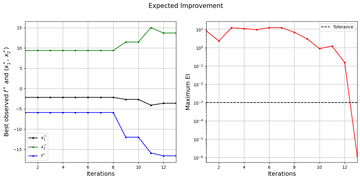
The figure on left shows the history of best observed \(y\) value and corresponding \(x\) values, and figure on right shows the convergence of EI. At the start, EI is high since the amount of possible improvement over the current best point is high. As the iterations progress, the best observed value reaches the global minimum and the EI decreases. Also, note that process stopped before reaching maximum number of infills since the convergence criteria was met.

Below code plots the infill points.

####################################### Plotting initial samples and infills

# Reshaping into grid
reshape_size = int(np.sqrt(num_plot))
X = xplot[:,0].reshape(reshape_size, reshape_size)
Y = xplot[:,1].reshape(reshape_size, reshape_size)
Z = yplot.reshape(reshape_size, reshape_size)

# Level
levels = np.linspace(-17, -5, 5)
levels = np.concatenate((levels, np.linspace(0, 30, 7)))
levels = np.concatenate((levels, np.linspace(35, 60, 5)))
levels = np.concatenate((levels, np.linspace(70, 300, 12)))

fig, ax = plt.subplots(figsize=(8,6))
CS=ax.contour(X, Y, Z, levels=levels, colors='k', linestyles='solid', alpha=0.5, zorder=-10)
ax.clabel(CS, inline=1, fontsize=8)
ax.scatter(xtrain[0:num_train,0], xtrain[0:num_train,1], c="red", label='Initial samples')
ax.scatter(xtrain[num_train:,0], xtrain[num_train:,1], c="black", label='Infills')
ax.plot(-3.689, 13.630, 'g*', markersize=15, label="Global minimum")
ax.plot(xbest[-1,0], xbest[-1,1], 'bo', label="Obtained minimum")
ax.legend()
ax.set_xlabel("$x_1$", fontsize=14)
ax.set_ylabel("$x_2$", fontsize=14)
ax.set_title("Modified Branin function", fontsize=15)

Text(0.5, 1.0, 'Modified Branin function')

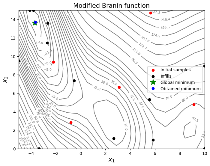
From the above plots, it can be seen that expected improvement finds the minimum of modified branin function while balancing exploration and exploitation.

NOTE: Due to randomness in differential evolution, results may vary slightly between runs. So, it is recommended to run the code multiple times to see average behavior.

Final result:

Parameter	True minimum	Obtained minimum
\(x_1^*\)	-3.689	-3.640
\(x_2^*\)	13.630	13.686
\(f(x_1^*, x_2^*)\)	-16.644	-16.601