Constrained Sequential Sampling

This section provides implementation for concepts related to constrained sequential sampling, refer lecture notes for more details. One of the ways to incorporate constraints in sequential sampling is to solve a constrained optimization problem to find the next infill point, instead an unconstrained optimization. All the methods covered in previous section can be used with this approach. In this section, only following methods are described:

1. Constrained Exploitation

2. Constrained Exploration

3. Constrained Expected Improvement

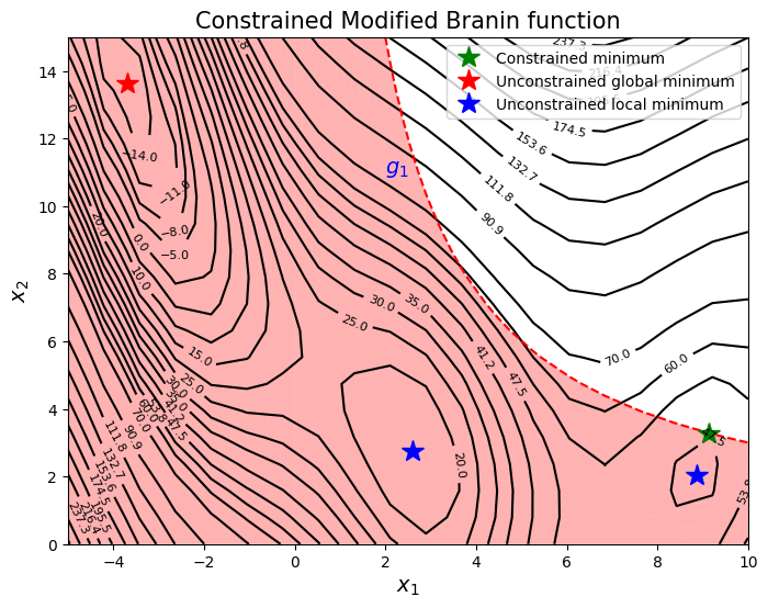
To demonstrate the working of these methods, constrained version of Modified Branin function, which is written as

\[\begin{split} \begin{gathered} f(x_1, x_2) = \Bigg ( x_2 - \frac{5.1}{4\pi^2} x_1^2 + \frac{5}{\pi}x_1 - 6 \Bigg)^2 + 10 \Bigg( 1-\frac{1}{8\pi} \Bigg)\cos x_1 + 10 + 5x_1 \\ g(x_1, x_2) = x_1x_2 \geq 30 \\ -5 \leq x_1 \leq 10 \text{ and } 0 \leq x_2 \leq 15, \end{gathered} \end{split}\]

is used as a test function. The constrained minimum is \(f(x^*) = 47.56\) at \(x^* = (9.143, 3.281)\). For demonstration, gaussian process models will be used. Below block of code defines the function and constraint.

import numpy as np
import matplotlib.pyplot as plt
from smt.sampling_methods import FullFactorial

def modified_branin(x):

    dim = x.ndim

    if dim == 1:
        x = x.reshape(1, -1)

    x1 = x[:,0]
    x2 = x[:,1]

    b = 5.1 / (4*np.pi**2)
    c = 5 / np.pi
    t = 1 / (8*np.pi)

    y = (x2 - b*x1**2 + c*x1 - 6)**2 + 10*(1-t)*np.cos(x1) + 10 + 5*x1

    if dim == 1:
        y = y.reshape(-1)

    return y

def constraint(x):

    dim = x.ndim

    if dim == 1:
        x = x.reshape(1, -1)

    x1 = x[:,0]
    x2 = x[:,1]

    g = -x1*x2 + 30
    
    if dim == 1:
        g = g.reshape(-1)

    return g

Below code plots the function, constraint and global minimum.

# Bounds
lb = np.array([-5, 10])
ub = np.array([0, 15])

# Plotting data
sampler = FullFactorial(xlimits=np.array([lb, ub]))
num_plot = 400
xplot = sampler(num_plot)
yplot = modified_branin(xplot)
gplot = constraint(xplot)

# Reshaping into grid
reshape_size = int(np.sqrt(num_plot))
X = xplot[:,0].reshape(reshape_size, reshape_size)
Y = xplot[:,1].reshape(reshape_size, reshape_size)
Z = yplot.reshape(reshape_size, reshape_size)
G = gplot.reshape(reshape_size, reshape_size)

# Level
levels = np.linspace(-17, -5, 5)
levels = np.concatenate((levels, np.linspace(0, 30, 7)))
levels = np.concatenate((levels, np.linspace(35, 60, 5)))
levels = np.concatenate((levels, np.linspace(70, 300, 12)))

fig, ax = plt.subplots(figsize=(8,6))

# Plot function
CS=ax.contour(X, Y, Z, levels=levels, colors='k', linestyles='solid')
ax.clabel(CS, inline=1, fontsize=8)

# Plot constraint
ax.contour(X, Y, G, levels=[0], colors='r', linestyles='dashed')
ax.contourf(X, Y, G, levels=np.linspace(0,G.max()), colors="red", alpha=0.3, antialiased = True)
ax.annotate('$g_1$', xy =(2.0, 11.0), fontsize=14, color='b')

# Plot minimum
ax.plot(9.143, 3.281, 'g*', markersize=15, label="Constrained minimum")
ax.plot(-3.689, 13.630, 'r*', markersize=15, label="Unconstrained global minimum")
ax.plot(2.594, 2.741, 'b*', markersize=15, label="Unconstrained local minimum")
ax.plot(8.877, 2.052,'b*', markersize=15)

# Asthetics
ax.set_xlabel("$x_1$", fontsize=14)
ax.set_ylabel("$x_2$", fontsize=14)
ax.set_title("Constrained Modified Branin function", fontsize=15)
ax.legend()

<matplotlib.legend.Legend at 0x7f6b8e73ad00>

The goal is to find minimum of the function while satisfying constraint using sequential sampling.