Multiobjective optimization using differential evolution

In the introduction, two multiobjective optimization problems were described and the Pareto fronts of the problems were found by sampling the space and using a non-dominated sorting algorithm that finds a set of non-dominated solutions within the sampled points. However, the sorting algorithm can find it harder to find accurate fronts in the case of problems with complex functions. In this section, the non-dominated sorting differential evolution (NSDE) algorithm is introduced and used to solve the same two optimization problems. This algorithm uses the non-dominated sorting method and applies it to each population of the differential evolution algorithm. That along with other heuristics such as crowding functions makes it more likely that the algorithm finds a more accurate Pareto front for a problem than just using the non-dominated sorting method.

NOTE: The NSDE algorithm used in this section has been implemented using pymoode which is an extension for pymoo and contains multiobjective differential evolution methods. pymoode must be installed before running the code of this section. To install it, activate your conda environment and use the command pip install pymoode==0.3.0rc3. Make sure that you use this exact command since other versions pymoode have certains bugs that prevent installation.

The block of code below imports the required packages for this section

import numpy as np
import matplotlib.pyplot as plt
from pymoo.core.problem import Problem
from pymoo.optimize import minimize
from pymoode.algorithms import NSDE
from pymoode.survival import RankAndCrowding
from pymoo.util.nds.non_dominated_sorting import NonDominatedSorting

Branin-Currin optimization problem

The Branin-Currin optimization problem was described in the previous section. The block of code below defines the two objective functions of the problem.

# Defining the objective functions
def branin(x):

    dim = x.ndim
    if dim == 1:
        x = x.reshape(1,-1)

    x1 = 15*x[:,0] - 5
    x2 = 15*x[:,1]

    b = 5.1 / (4*np.pi**2)
    c = 5 / np.pi
    t = 1 / (8*np.pi)

    y = (1/51.95)*((x2 - b*x1**2 + c*x1 - 6)**2 + 10*(1-t)*np.cos(x1) + 10 - 44.81)

    if dim == 1:
        y = y.reshape(-1)

    return y

def currin(x):

    dim = x.ndim
    if dim == 1:
        x = x.reshape(1,-1)

    x1 = x[:,0]
    x2 = x[:,1]
    
    factor = 1 - np.exp(-1/(2*x2))
    num = 2300*x1**3 + 1900*x1**2 + 2092*x1 + 60
    den = 100*x1**3 + 500*x1**2 + 4*x1 + 20
    y = factor*num/den
    
    if dim == 1:
        y = y.reshape(-1)

    return y

The blocks of code below defines the Problem class for the optimization problem. The optimization problem is solved using the NSDE algorithm that is given in pymoode. The number of generations and function evaluations required by the algorithm are also reported.

# Defining the problem class for pymoo - we are evaluating two objective functions in this case
class BraninCurrin(Problem):

    def __init__(self):
        super().__init__(n_var=2, n_obj=2, n_constr=0, xl=np.array([1e-6, 1e-6]), xu=np.array([1, 1]))

    def _evaluate(self, x, out, *args, **kwargs):

        out["F"] = np.column_stack((branin(x), currin(x)))

problem = BraninCurrin()
algorithm = NSDE(pop_size=100, CR=0.9, survival=RankAndCrowding(crowding_func="pcd"),save_history = True) 
res_nsde = minimize(problem, algorithm, verbose=False)
print("Number of generations:", len(res_nsde.history))
print("Number of function evaluations:", res_nsde.algorithm.evaluator.n_eval)

Number of generations: 95
Number of function evaluations: 9500

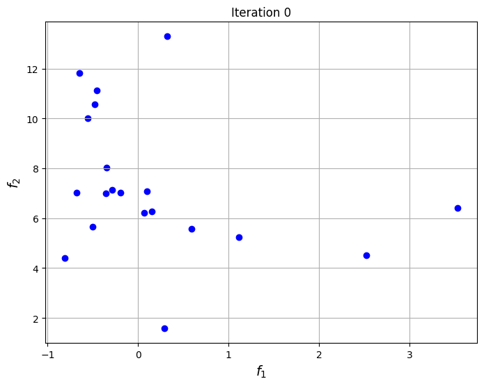
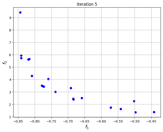
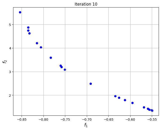
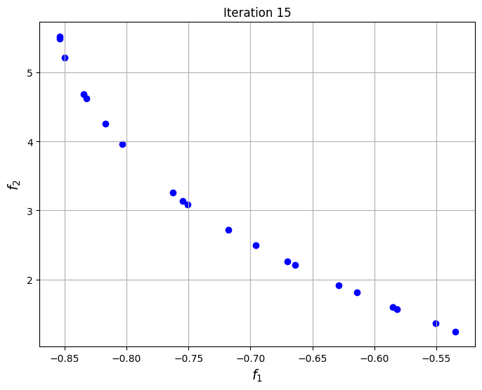
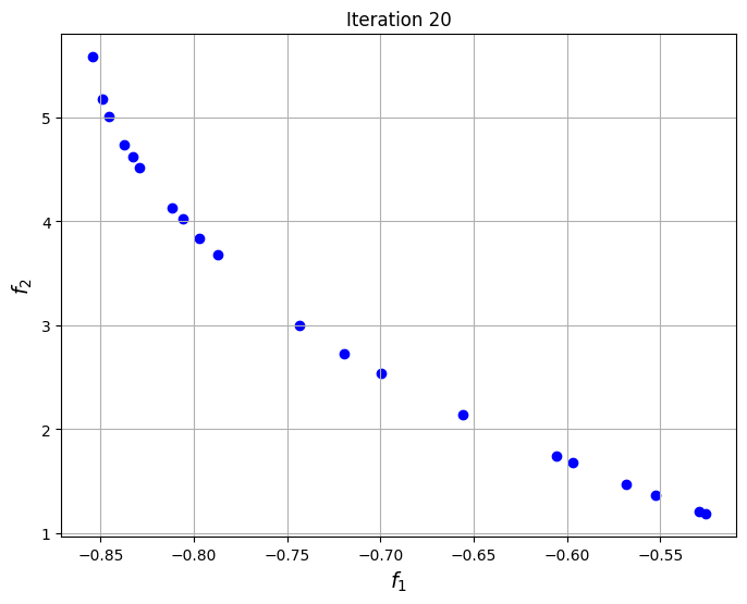
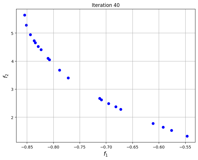
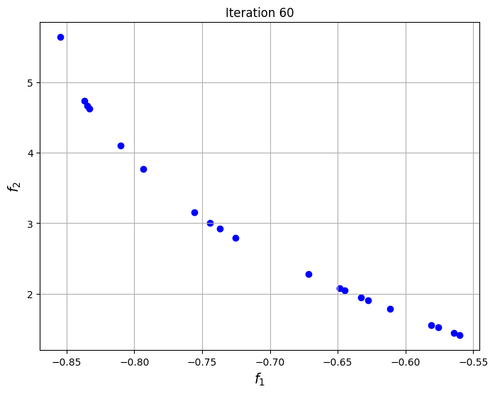
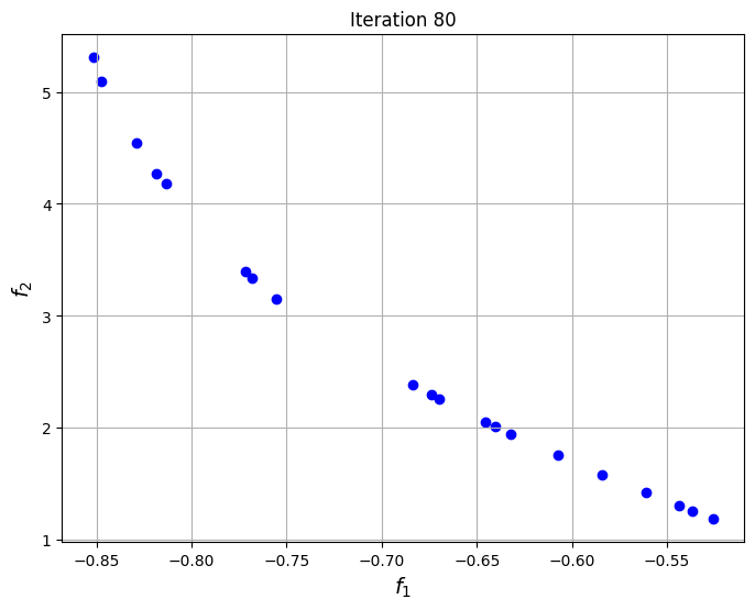
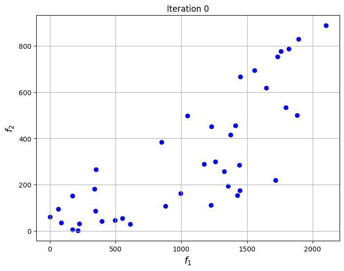
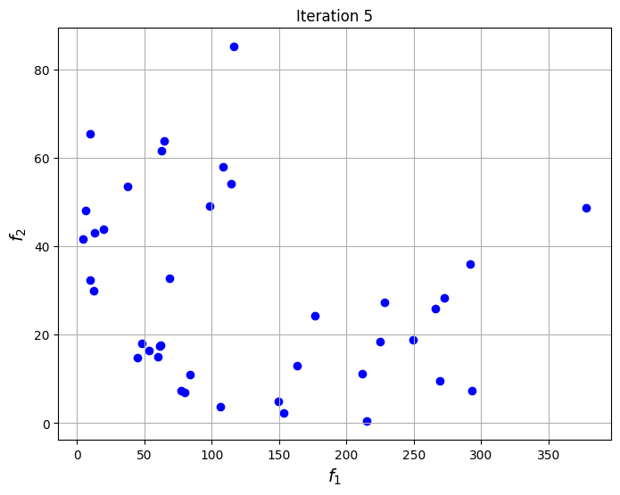
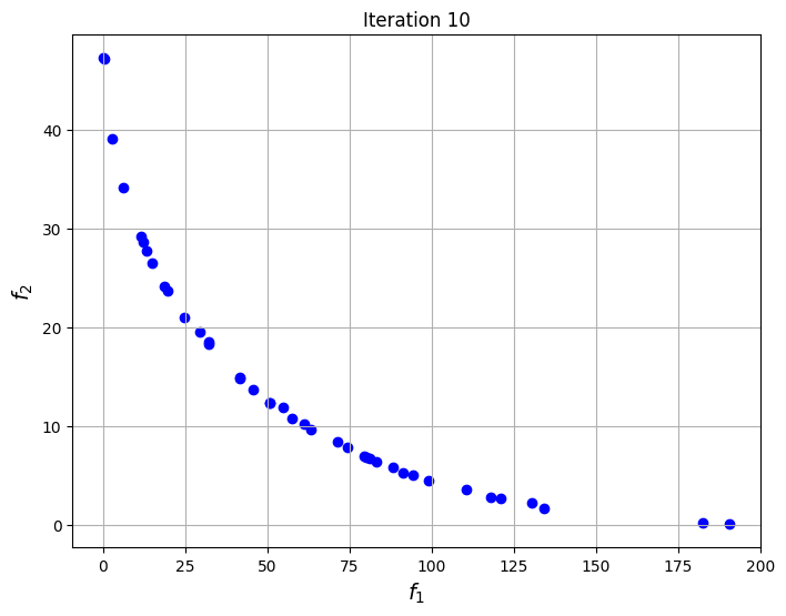
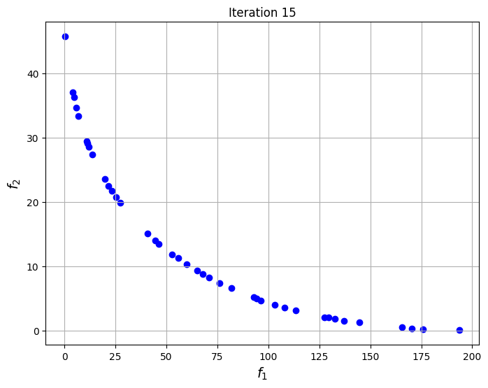
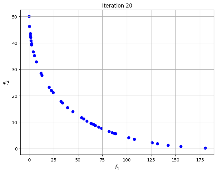
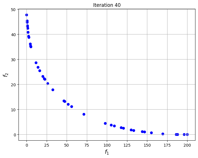
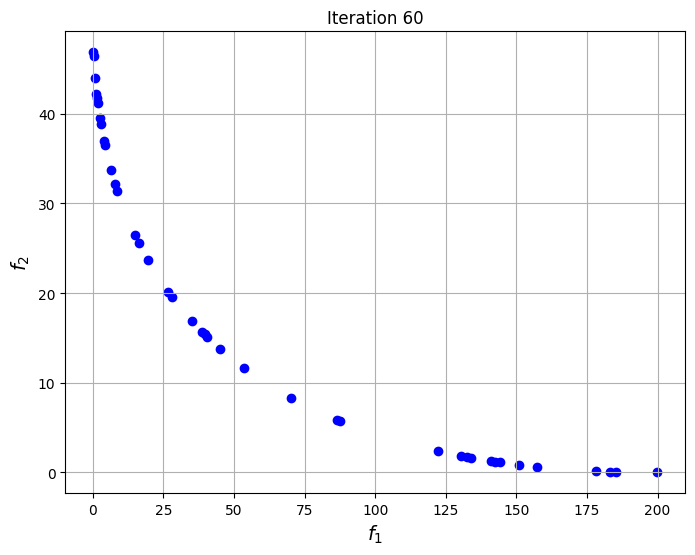
To visualize the convergence of the algorithm, the set of non-dominated points found at each generation of NSDE are plotted at specific iterations of the algorithm. The plots show that the set of non-dominated points converges to the Pareto front of the problem as the iterations progress.

niter = len(res_nsde.history) # Number of iterations
iterations = np.arange(0,20,5)
iterations = np.concatenate((iterations, np.arange(20,niter,20)))

# Plotting the particle evolution
for itr in iterations:
    fig, ax = plt.subplots(1,1,figsize = (8,6))
    ax.scatter(res_nsde.history[itr].pop.get("F")[::5, 0], res_nsde.history[itr].pop.get("F")[::5, 1], color = "blue")
    ax.set_title("Iteration %s" % itr)
    ax.grid()
    ax.set_xlabel("$f_1$", fontsize = 14)
    ax.set_ylabel("$f_2$", fontsize = 14)

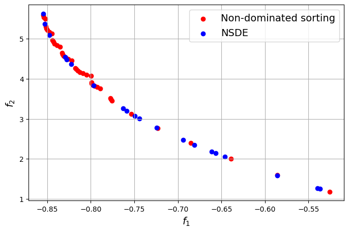
The block of code below plots the final Pareto front obtained for the problem and comapares it to the one found using non-dominated sorting alone. The Pareto front obtained using differential evolution is similar to the one obtained using non-dominated sorting, however, the known frontier of the problem is known to be smooth and this smoothness is better captured by the NSDE solution as compared to the non-dominated sorting solution.

# Generating a grid of points
num_points = 100

# Defining x and y values
x = np.linspace(1e-6,1,num_points)
y = np.linspace(1e-6,1,num_points)

# Creating a mesh
X, Y = np.meshgrid(x, y)

# Finding the front through non-dominated sorting
z1 = branin(np.hstack((X.reshape(-1,1),Y.reshape(-1,1))))
z2 =  currin(np.hstack((X.reshape(-1,1),Y.reshape(-1,1))))
nds = NonDominatedSorting()
F = np.column_stack((z1,z2))
pareto = nds.do(F, n_stop_if_ranked=50)
Z_pareto = F[pareto[0]]

# Plotting final Pareto frontier obtained
fig, ax = plt.subplots(figsize=(8, 5))
ax.scatter(Z_pareto[1:,0], Z_pareto[1:,1], color="red", label="Non-dominated sorting")
ax.scatter(res_nsde.F[::5, 0], res_nsde.F[::5, 1], color="blue", label="NSDE")
ax.set_ylabel("$f_2$", fontsize = 14)
ax.set_xlabel("$f_1$", fontsize = 14)
ax.legend(fontsize = 14)
ax.grid()

Constrained optimization problem

The constrained optimization problem was described in the previous section. The code block below defines the objective and constraint functions for the problem.

# Defining the objective functions
def f1(x):
    
    dim = x.ndim
    if dim == 1:
        x = x.reshape(1,-1)

    y = 4*x[:,0]**2 + 4*x[:,1]**2
    
    return y
    
def f2(x):

    dim = x.ndim
    if dim == 1:
        x = x.reshape(1,-1)

    y = (x[:,0]-5)**2 + (x[:,1]-5)**2

    return y

def g1(x):
    
    dim = x.ndim
    if dim == 1:
        x = x.reshape(1,-1)
    
    g = (x[:,0]-5)**2 + x[:,1]**2 - 25

    return g

def g2(x):

    dim = x.ndim
    if dim == 1:
        x = x.reshape(1,-1)
    
    g = 7.7 - ((x[:,0]-8)**2 + (x[:,1]+3)**2)

    return g

# Defining the problem class for pymoo - we are evaluating two objective and two constraint functions in this case
class ConstrainedProblem(Problem):

    def __init__(self):
        super().__init__(n_var=2, n_obj=2, n_ieq_constr=2, vtype=float)

        self.xl = np.array([-20.0, -20.0])
        self.xu = np.array([20.0, 20.0])

    def _evaluate(self, x, out, *args, **kwargs):

        out["F"] = np.column_stack([f1(x), f2(x)])
        out["G"] = np.column_stack([g1(x), g2(x)])

The blocks of code below defines the Problem class for the optimization problem. The optimization problem is solved using the NSDE algorithm that is given in pymoode. The number of generations and function evaluations required by the algorithm are also reported. The convergence of the process is shown by plotting the non-dominated solutions obtained at every iteration of the algorithm. This shows the evolution of the Pareto front as the iterations progress.

problem = ConstrainedProblem()
nsde = NSDE(pop_size=200, CR=0.8, survival=RankAndCrowding(crowding_func="pcd"), save_history = True)
res_nsde = minimize(problem, nsde, verbose=False)
print("Number of generations:", len(res_nsde.history))
print("Number of function evaluations:", res_nsde.algorithm.evaluator.n_eval)

Number of generations: 78
Number of function evaluations: 15600

niter = len(res_nsde.history) # Number of iterations
iterations = np.arange(0,20,5)
iterations = np.concatenate((iterations, np.arange(20,niter,20)))

# Plotting the particle evolution
for itr in iterations:
    fig, ax = plt.subplots(1,1,figsize = (8,6))
    ax.scatter(res_nsde.history[itr].pop.get("F")[::5, 0], res_nsde.history[itr].pop.get("F")[::5, 1], color = "blue")
    ax.set_title("Iteration %s" % itr)
    ax.grid()
    ax.set_xlabel("$f_1$", fontsize = 14)
    ax.set_ylabel("$f_2$", fontsize = 14)

# Generating a grid of points
num_points = 100

# Defining x and y values
x = np.linspace(-20,20,num_points)
y = np.linspace(-20,20,num_points)

# Creating a mesh
X, Y = np.meshgrid(x, y)

# Finding the front through non-dominated sorting
z1 = f1(np.hstack((X.reshape(-1,1),Y.reshape(-1,1))))
z2 = f2(np.hstack((X.reshape(-1,1),Y.reshape(-1,1))))
const1 = g1(np.hstack((X.reshape(-1,1),Y.reshape(-1,1))))
const2 = g2(np.hstack((X.reshape(-1,1),Y.reshape(-1,1))))
z1 = z1[(const1<0) & (const2<0)]
z2 = z2[(const1<0) & (const2<0)]
nds = NonDominatedSorting()
F = np.column_stack((z1,z2))
pareto = nds.do(F, n_stop_if_ranked=50)
Z_pareto = F[pareto[0]]

# Plotting final Pareto frontier obtained
fig, ax = plt.subplots(figsize=(8, 5))
ax.scatter(Z_pareto[:,0], Z_pareto[:,1], color="red", label="Non-dominated sorting")
ax.scatter(res_nsde.F[::5, 0], res_nsde.F[::5, 1], color="blue", label="NSDE")
ax.set_ylabel("$f_2$", fontsize = 14)
ax.set_xlabel("$f_1$", fontsize = 14)
ax.legend(fontsize = 14)
ax.grid()

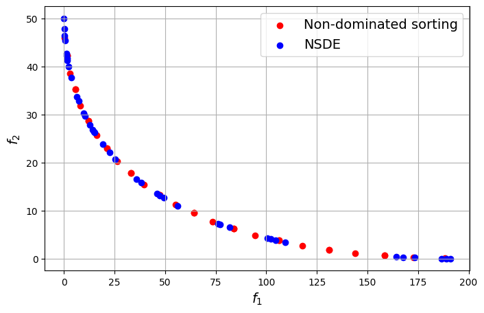
In this case, the Pareto front obtained using the non-dominated sorting algorithm and the NSDE algorithm are identical to each other. This means that when the functions of the problem are simple enough, both direct sorting of the solutions and directly solving the optimization problems will yield similar results. The Pareto front for this problem is a smooth convex curve.