Sequential Sampling using Dimensionality Reduction

This section provides an example implementation of the usage of dimensionality reduction along with expected improvement (EI) to perform exploration and exploitation of a high-dimensional function. The dimensionality reduction methods used in this section are principal component analysis (PCA) and kernel principal component analysis. The example problem used to demonstrate sequential sampling using dimensionality reduction is the 10-dimensional Styblinski-Tang function. The problem statement can be written as

\[f(\textbf{x}) = \frac{1}{2} \sum_{i=1}^{10} (x_i^4 - 16x_i^2 + 5x_i)\]

\[ -5 \leq x_i \leq 5, \quad i = 1,...,10 \]

The global minimum of the function is \(f(\textbf{x}^*)=-391.6599\) at \(\textbf{x}^*=(-2.904,...,-2.904)\).

# Imports
import numpy as np
import time
from sklearn.decomposition import PCA, KernelPCA
from smt.surrogate_models import KRG
from smt.sampling_methods import LHS
import matplotlib.pyplot as plt
from pymoo.core.problem import Problem
from pymoo.algorithms.soo.nonconvex.de import DE
from pymoo.optimize import minimize
from pymoo.config import Config
Config.warnings['not_compiled'] = False
from scipy.stats import norm as normal

The block of code below defines the Styblinski-Tang function for any number of dimensions. We will be using the 10-dimensional version of the function and therefore, need to provide a 10-dimensional input to this function.

# Styblinski-Tang function
def f(x):
    """
        Function which calculates the Styblinski-Tang function value at given x.
        
        Input:
        x - 1D/2D numpy array
    """

    # Number of dimensions of input
    dim = x.ndim

    # To ensure n x 2
    if dim == 1:
        x = x.reshape(1,-1)

    innersum = np.zeros((x.shape[0], x.shape[1], 3))

    innersum[:,:,0] = x**4
    innersum[:,:,1] = -16*x**2
    innersum[:,:,2] = 5*x

    outersum = np.sum(innersum, axis=2)
    
    y = 0.5*np.sum(outersum, axis=1, keepdims=True)
    
    if dim == 1:
        y = y.reshape(-1,)
    
    return y

Sequential Sampling using Expected Improvement (EI)

The blocks of code below will perform sequential sampling using the standard EI that was demonstrated in the Sequential Sampling section of the Jupyter Book. The random state for the generation of initial samples is fixed since the results obtained using EI will be compared to those obtained using the dimensionality reduction methods and therefore, it is important for each of the algorithms to start with the same initial samples. However, the results can still vary if the sequential sampling is re-run since the seed for differential evolution has not been set. For a fair comparison, the convergence criterion of the sampling is set as the maximum number of iterations. This is so that EI and the other methods will run for the same number of iterations and perform the same number of infills. In the end, the best objective value can be compared to compare the performance of the algorithms. As you will observe, it is also quite difficult for the max EI to meet the convergence criteria for a high-dimensional function. In such cases, the aim is to obtain the best possible value of the objective function in the shortest amount of sampling iterations.

# Setting number of dimensions for the problem - 10D Styblinski-Tang Function
ndim = 10

# Defining bounds
lb = np.array([-5]*ndim)
ub = np.array([5]*ndim)
    
# Problem class
class EI(Problem):

    def __init__(self, sm, ymin):
        super().__init__(n_var=ndim, n_obj=1, n_constr=0, xl=lb, xu=ub)

        self.sm = sm # store the surrogate model
        self.ymin = ymin

    def _evaluate(self, x, out, *args, **kwargs):

        # Standard normal
        numerator = self.ymin - self.sm.predict_values(x)
        denominator = np.sqrt( self.sm.predict_variances(x) )
        z = numerator / denominator
        
        # Computing expected improvement
        # Negative sign because we want to maximize EI
        out["F"] = - ( numerator * normal.cdf(z) + denominator * normal.pdf(z) )

# Optimization algorithm
algorithm = DE(pop_size=100, CR=0.8, dither="vector")

The block of code below creates 20 training points and performs the sequential sampling process using EI. The convergence criterion is set at a maximum number of 45 iterations.

# Setting a random state to allow a fair comparison between the different methods
random_state = 20
xlimits = np.column_stack((lb,ub))
sampler = LHS(xlimits=xlimits, criterion='ese', random_state = 20)

# Training data
num_train = 20
xtrain = sampler(num_train)
ytrain = f(xtrain)

# Variables
itr = 0
max_itr = 45
tol = 1e-3
max_EI = [1]
ybest = []
corr = 'squar_exp'
fs = 12

# Sequential sampling Loop
t1 = time.time()
while itr < max_itr:
        
    print("\nIteration {}".format(itr + 1))

    # Initializing the kriging model
    sm = KRG(theta0=[1e-2], corr=corr, theta_bounds=[1e-6, 1e2], print_global=False)

    # Setting the training values
    sm.set_training_values(xtrain, ytrain)
    
    # Creating surrogate model
    sm.train()

    # Find the best observed sample
    ybest.append(np.min(ytrain))

    # Find the minimum of surrogate model
    result = minimize(EI(sm, ybest[-1]), algorithm, verbose=False)
    
    # Computing true function value at infill point
    y_infill = f(result.X.reshape(1,-1))

    # Storing variables
    if itr == 0:
        max_EI[0] = -result.F[0]
        xbest = xtrain[np.argmin(ytrain)].reshape(1,-1)
    else:
        max_EI.append(-result.F[0])
        xbest = np.vstack((xbest, xtrain[np.argmin(ytrain)]))

    print("Maximum EI: {}".format(max_EI[-1]))
    print("Best observed value: {}".format(ybest[-1]))

    # Appending the the new point to the current data set
    xtrain = np.vstack(( xtrain, result.X.reshape(1,-1) ))
    ytrain = np.append( ytrain, y_infill )
    
    itr = itr + 1 # Increasing the iteration number

t2 = time.time()
# Printing the final results
print("\nBest obtained point:")
print("x*: {}".format(xbest[-1]))
print("f*: {}".format(ybest[-1]))

# Storing results
ei_ybest = ybest
ei_xbest = xbest
ei_time = t2 - t1

Iteration 1
Maximum EI: 29.9348389478
Best observed value: -150.53602901269912

Iteration 2
Maximum EI: 14.313598360026237
Best observed value: -150.53602901269912

Iteration 3
Maximum EI: 22.179316153376632
Best observed value: -150.53602901269912

Iteration 4
Maximum EI: 47.68078740723258
Best observed value: -150.53602901269912

Iteration 5
Maximum EI: 27.92762674314964
Best observed value: -150.53602901269912

Iteration 6
Maximum EI: 35.52459213127647
Best observed value: -150.53602901269912

Iteration 7
Maximum EI: 21.340778116409087
Best observed value: -192.73791154099587

Iteration 8
Maximum EI: 31.383882396972645
Best observed value: -192.73791154099587

Iteration 9
Maximum EI: 100.85633714502279
Best observed value: -192.73791154099587

Iteration 10
Maximum EI: 122.32202034153798
Best observed value: -192.73791154099587

Iteration 11
Maximum EI: 80.8309296006207
Best observed value: -192.73791154099587

Iteration 12
Maximum EI: 31.260095296453123
Best observed value: -192.73791154099587

Iteration 13
Maximum EI: 151.88959638844773
Best observed value: -192.73791154099587

Iteration 14
Maximum EI: 157.57438822132775
Best observed value: -192.73791154099587

Iteration 15
Maximum EI: 35.026518026884695
Best observed value: -253.5774800946036

Iteration 16
Maximum EI: 40.05880408843345
Best observed value: -253.5774800946036

Iteration 17
Maximum EI: 58.57645237370734
Best observed value: -253.5774800946036

Iteration 18
Maximum EI: 19.833993204779233
Best observed value: -253.5774800946036

Iteration 19
Maximum EI: 53.998707036136615
Best observed value: -253.5774800946036

Iteration 20
Maximum EI: 35.433099424032086
Best observed value: -253.5774800946036

Iteration 21
Maximum EI: 141.66355228032603
Best observed value: -253.5774800946036

Iteration 22
Maximum EI: 61.554321842411575
Best observed value: -253.5774800946036

Iteration 23
Maximum EI: 24.163608795294632
Best observed value: -253.5774800946036

Iteration 24
Maximum EI: 34.46314298786474
Best observed value: -253.5774800946036

Iteration 25
Maximum EI: 47.58428938642727
Best observed value: -253.5774800946036

Iteration 26
Maximum EI: 73.62714098837189
Best observed value: -253.5774800946036

Iteration 27
Maximum EI: 65.15735444189076
Best observed value: -253.5774800946036

Iteration 28
Maximum EI: 35.8420833840719
Best observed value: -253.5774800946036

Iteration 29
Maximum EI: 40.774785212229574
Best observed value: -253.5774800946036

Iteration 30
Maximum EI: 105.86959520012738
Best observed value: -253.5774800946036

Iteration 31
Maximum EI: 26.743519409189027
Best observed value: -253.5774800946036

Iteration 32
Maximum EI: 59.27164708421749
Best observed value: -253.5774800946036

Iteration 33
Maximum EI: 16.777867763941636
Best observed value: -253.5774800946036

Iteration 34
Maximum EI: 103.14344593068768
Best observed value: -253.5774800946036

Iteration 35
Maximum EI: 38.507210472613274
Best observed value: -253.5774800946036

Iteration 36
Maximum EI: 83.84116152222884
Best observed value: -253.5774800946036

Iteration 37
Maximum EI: 45.98842872492748
Best observed value: -253.5774800946036

Iteration 38
Maximum EI: 40.16082675619078
Best observed value: -253.5774800946036

Iteration 39
Maximum EI: 59.16649503409608
Best observed value: -253.5774800946036

Iteration 40
Maximum EI: 60.47936286860907
Best observed value: -253.5774800946036

Iteration 41
Maximum EI: 45.26394341491553
Best observed value: -253.5774800946036

Iteration 42
Maximum EI: 17.117510644528192
Best observed value: -253.5774800946036

Iteration 43
Maximum EI: 14.92894101279543
Best observed value: -253.5774800946036

Iteration 44
Maximum EI: 42.15794217533398
Best observed value: -253.5774800946036

Iteration 45
Maximum EI: 19.85722675846832
Best observed value: -253.5774800946036

Best obtained point:
x*: [-1.40635186 -2.74523788 -2.42496525 -0.71897207 -1.25984989 -2.97299565
 -1.70697381 -2.84230564 -2.82505042 -0.17037821]
f*: -253.5774800946036

The block of code below will plot the history of the best observed value of the objective function against the number of iterations.

# Plotting variation of best value of objective function
fig, ax = plt.subplots(1, 1, figsize=(14,6))
ax.plot(np.arange(itr) + 1, ei_ybest, c="blue", label='EI', marker=".")
ax.set_xlabel("Iterations", fontsize=14)
ax.set_ylabel("Best observed $f^*$", fontsize=14)
ax.legend(fontsize = 14)
ax.set_xlim(left=1, right=itr)
ax.grid()

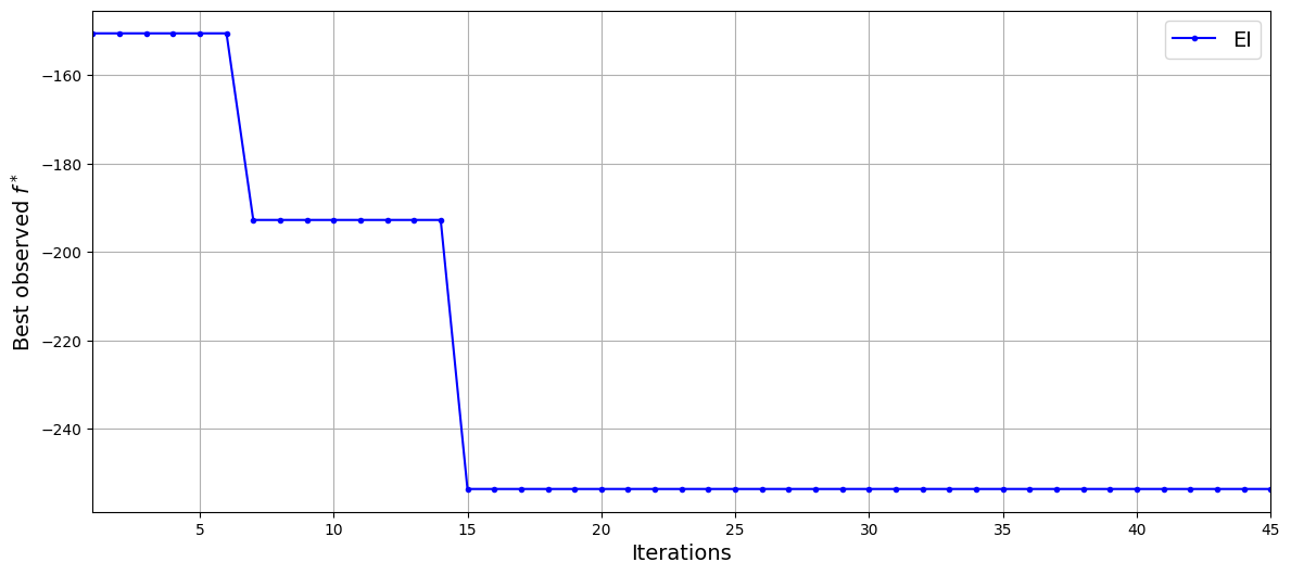
The results of EI show that the sequential sampling algorithm is not able to find the global optimum of the function even after the addition of 45 infill samples. This is demonstrative of the difficulty of optimizing high-dimensional functions using surrogate-based methods. However, the algorithm is able to decrease the best observed value of the function from aporoximately -150 to approximately -253. Now, the same problem will be solved using dimensionality reduction methods to demonstrate the improvements that can be seen while optimizing high-dimensional functions.

Sequential Sampling using Pricinpal Component Analysis and EI (PCA-EI)

The blocks of code below will demonstrate the use of PCA along with EI to optimize the function using sequential sampling. The main idea here is to reduce the dimensionality of the input data from 10 to 5 using PCA. The 5 principal components obtained in this manner will be the new design variables for the problem. The kriging model will use the principal components as the input data and the original function values as the output data. Essentially, this means that we will be solving a new optimization problem that has lower dimensionality than the original 10-dimensional problem. In this case, the optimization problem statement for maximizing EI has to be redefined as

\[\begin{split}\underset{\xi}{\max} \text{PEI}(\xi) = \begin{cases} \text{EI}(\xi) & \xi \; \textrm{is feasible}\\ -P & \xi \; \textrm{is infeasible} \end{cases} \end{split}\]

\[ \min(\xi_i) \leq \xi_i \leq \max(\xi_i), \quad i = 1,...,5 \]

where \(\xi\) represents the principal components found using PCA and \(\text{PEI}(\xi)\) represents the penalized version of EI. The bounds for the maximization are the maximum and minimum values of \(\xi\) that are found using the sampling plan at a given iteration of the sequential sampling algorithm. Even though bounds are placed on the low-dimensional representation of the problem using the minimum and maximum values of the principal components, the usage of penalized expected improvement is required since it is not known that the point evaluated by differential evolution while maximizing the penalized EI actually lies within the bounds of the original problem. It is, therefore, necessary to penalize the points that are outside of the original bounds of the problem. At each evaluation of the objective in differential evolution, the principal components are transformed back to the original high-dimensional space and a check is performed to determine if the point being evaluated is within the bounds of the original problem or not. If it is within the original bounds, then the objective returns the standard EI otherwise it will return a large value as a penalty. In this case, the penalty, P, is a fixed value of 1000, however, more intricate implementations could vary the penalty based on the point in the design space being evaluated.

Additionally, an important parameter for PCA is the number of principal components to use, which must be selected by the user. To determine the correct number of principal components, the cumulative explained variance ratio plot described in the previous section can be used. The block of code below plots the cumulative explained variance ratio plot for the 10-dimensional Styblinksi-Tang function.

# Generating data
xlimits = np.column_stack((lb,ub))
random_state = 20
sampler = LHS(xlimits=xlimits, criterion='ese', random_state=random_state)

num_train = 50
xtrain = sampler(num_train)
ytrain = f(xtrain)

# Pre-processing data before applying PCA
center = xtrain.mean(axis = 0)
xtrain_center = xtrain - center

# Calculating sum of explained variance ratios
sum_explained_variance_ratio_ = []
n_components = np.arange(1,ndim+1,1)

for component in n_components:
    # Applying PCA to the data
    transform = PCA(n_components=component)
    xprime = transform.fit_transform(xtrain_center)
    sum_explained_variance_ratio_.append(np.sum(transform.explained_variance_ratio_))

fig, ax = plt.subplots(1, 1, figsize=(8,6))
ax.plot(n_components, sum_explained_variance_ratio_, marker='.')
ax.grid()
ax.set_xlabel('Number of Principal Components', fontsize = 14)
ax.set_ylabel('Cumulative Explained Variance Ratio', fontsize = 14)

Text(0, 0.5, 'Cumulative Explained Variance Ratio')

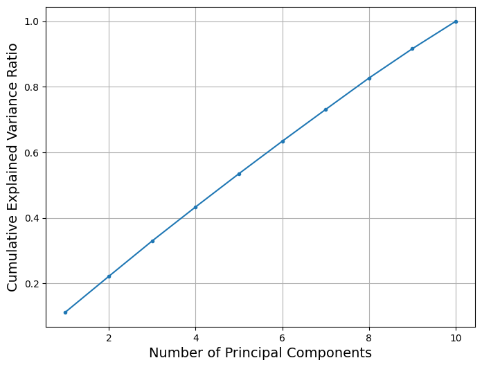
The above plot of the cumulative explained variance ratio shows that the cumulative explained variance ratio increases linearly with the number of principal components. This suggests that each of the design variables explains an equal ratio of the variance of the objective function and to satisfy a threshold of 95% cumulative explained variance ratio it will be necessary to select all of the principal components. However, in order to demonstrate the use of dimensionality reduction, five principal components are chosen to represent the objective function. This allows the representation of at least 50% of the variance in the objective which is enough to aid in optimizing the objective function of interest for this section. This will be made clear in the results of the sequential sampling that follow.

To begin the implementation of sequential sampling using PCA and EI, the block of code below defines the Problem class and differential evolution algorithm for the penalized EI that is to be used for sequential sampling using dimensionality reduction.

# Problem class
# Upper bound, lower bound and number of variables are added as parameters
class EI_DR(Problem):

    def __init__(self, sm, ymin, lb, ub, n_var, pca, center):
        super().__init__(n_var=n_var, n_obj=1, n_constr=0, xl=lb, xu=ub)

        self.sm = sm # store the surrogate model
        self.ymin = ymin
        self.pca = pca
        self.center = center
        
    def expected_improvement(self, x):
        
        numerator = self.ymin - self.sm.predict_values(x)
        denominator = np.sqrt( self.sm.predict_variances(x) )
        z = numerator / denominator
        
        return numerator * normal.cdf(z) + denominator * normal.pdf(z)
    
    def penalized_expected_improvement(self, x):
        
        # map back the candidate point to check if it falls inside the original domain
        x_ = self.pca.inverse_transform(x) + self.center
        idx_lower = np.where(x_ < -5.0)
        idx_lower = np.column_stack((idx_lower[0], idx_lower[1]))
        idx_upper = np.where(x_ > 5.0)
        idx_upper = np.column_stack((idx_upper[0], idx_upper[1]))
        
        out = self.expected_improvement(x)
        
        # Assigning a high valued penalty for points that are outside the original bounds of the 
        # problem
        out[idx_lower] = -1000
        out[idx_upper] = -1000

        return out

    def _evaluate(self, x, out, *args, **kwargs):
        
        # Computing expected improvement
        # Negative sign because we want to maximize EI
        out["F"] = - self.penalized_expected_improvement(x) 

# Optimization algorithm
algorithm = DE(pop_size=100, CR=0.8, dither="vector")

The block of code below creates 20 training points using the same random state as EI and performs the sequential sampling process using dimensionality reduction and EI. The convergence criterion is set at a maximum number of 45 iterations. At every iteration of the sequential sampling, the data is centered using the mean value. After that, PCA is performed at every iteration of the sampling to reduce the dimensionality of the EI maximization problem using the existing sampling plan at that iteration.

random_state = 20
sampler = LHS(xlimits=xlimits, criterion='ese', random_state=random_state)

# Training data
num_train = 20
xtrain = sampler(num_train)
ytrain = f(xtrain)

# Variables
itr = 0
max_itr = 45
tol = 1e-3
max_EI = [1]
ybest = []
corr = 'squar_exp'
fs = 12

# Sequential sampling Loop
t1 = time.time()
while itr < max_itr:
    
    print("\nIteration {}".format(itr + 1))
    
    # Pre-processing data before applying PCA
    center = xtrain.mean(axis = 0)
    xtrain_center = xtrain - center 

    # Applying PCA to the data
    transform = PCA(n_components=5)
    xprime = transform.fit_transform(xtrain_center)

    # Defining the bounds as the maximum and minimum value of the PC
    lb = xprime.min(axis = 0)
    ub = xprime.max(axis = 0)

    # Initializing the kriging model
    sm = KRG(theta0=[1e-2], corr=corr, theta_bounds=[1e-6, 1e2], print_global=False)

    # Setting the training values
    sm.set_training_values(xprime, ytrain)
    
    # Creating surrogate model
    sm.train()

    # Find the best observed sample
    ybest.append(np.min(ytrain))

    # Find the minimum of surrogate model
    result = minimize(EI_DR(sm, ybest[-1], lb=lb, ub=ub, n_var = xprime.shape[1], pca = transform, center = center), 
                      algorithm, verbose=False)
    
    # Inverse transform to the real space
    inverse_X = transform.inverse_transform(result.X.reshape(1,-1)) + center
    
    # Computing true function value at infill point
    y_infill = f(inverse_X)

    # Storing variables
    if itr == 0:
        max_EI[0] = -result.F[0]
        xbest = xtrain[np.argmin(ytrain)].reshape(1,-1)
    else:
        max_EI.append(-result.F[0])
        xbest = np.vstack((xbest, xtrain[np.argmin(ytrain)]))

    print("Maximum EI: {}".format(max_EI[-1]))
    print("Best observed value: {}".format(ybest[-1]))
    
    # Appending the the new point to the current data set
    xtrain = np.vstack(( xtrain, inverse_X ))
    ytrain = np.append( ytrain, y_infill )
    
    itr = itr + 1 # Increasing the iteration number

t2 = time.time()
# Printing the final results
print("\nBest obtained point:")
print("x*: {}".format(xbest[-1]))
print("f*: {}".format(ybest[-1]))

# Storing results
pca_xbest = xbest
pca_ybest = ybest
pca_time = t2 - t1

Iteration 1
Maximum EI: 8.101206122176006
Best observed value: -150.53602901269912

Iteration 2
Maximum EI: 24.35809591219134
Best observed value: -205.46718541728967

Iteration 3
Maximum EI: 9.274252846344787
Best observed value: -205.46718541728967

Iteration 4
Maximum EI: 13.081990715579746
Best observed value: -205.46718541728967

Iteration 5
Maximum EI: 12.99963681917075
Best observed value: -205.46718541728967

Iteration 6
Maximum EI: 16.895842823596272
Best observed value: -205.46718541728967

Iteration 7
Maximum EI: 7.9357712652656325
Best observed value: -205.46718541728967

Iteration 8
Maximum EI: 4.99776176110562
Best observed value: -225.37927694788365

Iteration 9
Maximum EI: 5.00937171312586
Best observed value: -225.37927694788365

Iteration 10
Maximum EI: 3.573573071987613
Best observed value: -243.41727796602

Iteration 11
Maximum EI: 2.234177460314492
Best observed value: -245.7420784175569

Iteration 12
Maximum EI: 0.12434559894876973
Best observed value: -245.7420784175569

Iteration 13
Maximum EI: 27.17989512087082
Best observed value: -245.7420784175569

Iteration 14
Maximum EI: 14.08936127746008
Best observed value: -245.7420784175569

Iteration 15
Maximum EI: 4.552937454559284
Best observed value: -245.7420784175569

Iteration 16
Maximum EI: 5.0849444909157135
Best observed value: -245.7420784175569

Iteration 17
Maximum EI: 3.309025588655839
Best observed value: -245.7420784175569

Iteration 18
Maximum EI: 0.9354759041253691
Best observed value: -247.9265027016814

Iteration 19
Maximum EI: 0.2393403896653158
Best observed value: -247.9265027016814

Iteration 20
Maximum EI: 2.853202401337315
Best observed value: -254.841398235717

Iteration 21
Maximum EI: 11.481467859901358
Best observed value: -254.841398235717

Iteration 22
Maximum EI: 2.558823925168365
Best observed value: -254.841398235717

Iteration 23
Maximum EI: 0.026359934505476745
Best observed value: -257.8409601836845

Iteration 24
Maximum EI: 0.41275928343689605
Best observed value: -257.8409601836845

Iteration 25
Maximum EI: 0.21985108615033
Best observed value: -257.8409601836845

Iteration 26
Maximum EI: 4.458964104408812
Best observed value: -257.8409601836845

Iteration 27
Maximum EI: 0.3081879682758799
Best observed value: -262.1085336224983

Iteration 28
Maximum EI: 4.224008282030557
Best observed value: -262.1085336224983

Iteration 29
Maximum EI: 0.19209213753520826
Best observed value: -262.1085336224983

Iteration 30
Maximum EI: 0.1760287266207199
Best observed value: -262.1085336224983

Iteration 31
Maximum EI: 8.29983652404847
Best observed value: -262.1085336224983

Iteration 32
Maximum EI: 2.4104678483884907
Best observed value: -265.88951388566846

Iteration 33
Maximum EI: 0.16276928526318946
Best observed value: -266.59429227358214

Iteration 34
Maximum EI: 0.22549808144920158
Best observed value: -266.59429227358214

Iteration 35
Maximum EI: 0.08170629696069798
Best observed value: -266.59429227358214

Iteration 36
Maximum EI: 0.3599060369250118
Best observed value: -266.59429227358214

Iteration 37
Maximum EI: 0.0873100806710364
Best observed value: -266.59429227358214

Iteration 38
Maximum EI: 2.932988638532323
Best observed value: -266.59429227358214

Iteration 39
Maximum EI: 0.1741619436658024
Best observed value: -266.59429227358214

Iteration 40
Maximum EI: 0.16207109431041555
Best observed value: -266.59429227358214

Iteration 41
Maximum EI: 0.05983065926832676
Best observed value: -266.59429227358214

Iteration 42
Maximum EI: 0.08228169101967442
Best observed value: -266.59429227358214

Iteration 43
Maximum EI: 0.13159592646475393
Best observed value: -266.59429227358214

Iteration 44
Maximum EI: 0.15753894225959075
Best observed value: -266.59429227358214

Iteration 45
Maximum EI: 0.8041647494370316
Best observed value: -266.59429227358214

Best obtained point:
x*: [-0.45588116 -0.68261111 -2.95021739 -1.43089789 -2.78725931  2.65876705
 -2.77834678 -3.36882078 -2.93935834  2.87592376]
f*: -266.59429227358214

# Plotting and comparing variation of best value of objective function
fig, ax = plt.subplots(1, 1, figsize=(12,6))
ax.plot(np.arange(itr) + 1, ei_ybest, c="blue", label='EI', marker=".")
ax.plot(np.arange(itr) + 1, ybest, c="red", label='PCA-EI', marker=".")
ax.set_xlabel("Iterations", fontsize=14)
ax.set_ylabel("Best observed $f^*$", fontsize=14)
ax.legend(fontsize = 14)
ax.set_xlim(left=1, right=itr)
ax.grid()

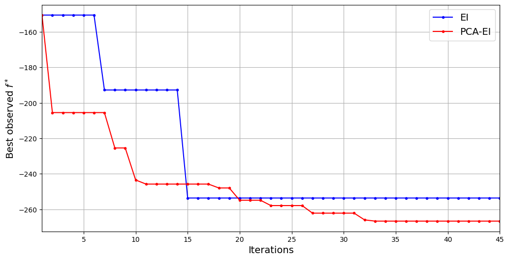
The above comparison of the best observed function values shows that sequential sampling using PCA provides a benefit over standard EI. It can reduce the best observed function value to approximately -266 which is a greater reduction than standard EI within the same number of maximum iterations. It can also be seen that in this particular run, PCA-EI also reduces the objective function quicker than standard EI. PCA-EI can produce a great reduction in the best observed function value as soon as 10 iterations while it can take standard EI 15 iterations to produce a comparable reduction in the best observed function value.

Sequential Sampling using Kernel PCA and EI (KPCA-EI)

The blocks of code below will demonstrate the use of Kernel PCA along with EI to optimize the function using sequential sampling. The idea is the same as PCA-EI and the dimensionality of the problem is reduced from 10 to 5 in this case as well. Penalized EI is used to find the new infill point and the parameters of the sampling are identical to those used for EI and PCA-EI. The difference lies in using Kernel PCA as a dimensionality reduction technique. Kernel PCA is a non-linear dimensionality reduction technique often performing better than PCA. However, it is important to correctly choose the hyperparameters of the Kernel PCA algorithm to ensure the best possible performance. Out of these, the most important hyperparameter is the choice of the kernel and other hyperparameters depend on which kernel is chosen for the algorithm. For this demonstration here, the hyperparameters are chosen as the default values with the kernel choice being the cosine kernel. In general, a procedure such as cross-validation can be used to find the best hyperparameters.

random_state = 20
sampler = LHS(xlimits=xlimits, criterion='ese', random_state=random_state)

# Training data
num_train = 20
xtrain = sampler(num_train)
ytrain = f(xtrain)

# Variables
itr = 0
max_itr = 45
tol = 1e-3
max_EI = [1]
ybest = []
corr = 'squar_exp'
fs = 12

# Sequential sampling Loop
t1 = time.time()
while itr < max_itr:
    
    print("\nIteration {}".format(itr + 1))
    
    # Pre-processing data before applying KPCA
    center = xtrain.mean(axis = 0)
    xtrain_center = xtrain - center 

    # Applying KPCA to the data
    transform = KernelPCA(n_components=5, kernel='cosine', fit_inverse_transform=True)
    xprime = transform.fit_transform(xtrain_center)
    
    # Defining the bounds as the maximum and minimum value of the PC
    lb = xprime.min(axis = 0)
    ub = xprime.max(axis = 0)

    # Initializing the kriging model
    sm = KRG(theta0=[1e-2], corr=corr, theta_bounds=[1e-6, 1e2], print_global=False)

    # Setting the training values
    sm.set_training_values(xprime, ytrain)
    
    # Creating surrogate model
    sm.train()

    # Find the best observed sample
    ybest.append(np.min(ytrain))

    # Find the minimum of surrogate model
    result = minimize(EI_DR(sm, ybest[-1], lb=lb, ub=ub, n_var = xprime.shape[1], pca = transform, center = center), 
                      algorithm, verbose=False)
    
    # Inverse transform to the real space
    inverse_X = transform.inverse_transform(result.X.reshape(1,-1)) + center
    
    # Computing true function value at infill point
    y_infill = f(inverse_X)

    # Storing variables
    if itr == 0:
        max_EI[0] = -result.F[0]
        xbest = xtrain[np.argmin(ytrain)].reshape(1,-1)
    else:
        max_EI.append(-result.F[0])
        xbest = np.vstack((xbest, xtrain[np.argmin(ytrain)]))

    print("Maximum EI: {}".format(max_EI[-1]))
    print("Best observed value: {}".format(ybest[-1]))
    
    # Appending the the new point to the current data set
    xtrain = np.vstack(( xtrain, inverse_X ))
    ytrain = np.append( ytrain, y_infill )
    
    itr = itr + 1 # Increasing the iteration number

t2 = time.time()
# Printing the final results
print("\nBest obtained point:")
print("x*: {}".format(xbest[-1]))
print("f*: {}".format(ybest[-1]))

# Storing time cost results
kpca_time = t2 - t1

Iteration 1
Maximum EI: 6.979328418587719
Best observed value: -150.53602901269912

Iteration 2
Maximum EI: 14.658139415927149
Best observed value: -170.46470349227047

Iteration 3
Maximum EI: 20.1589800042305
Best observed value: -170.46470349227047

Iteration 4
Maximum EI: 23.678652636989206
Best observed value: -170.46470349227047

Iteration 5
Maximum EI: 22.333801998614614
Best observed value: -184.02537973814339

Iteration 6
Maximum EI: 11.787397259763061
Best observed value: -184.02537973814339

Iteration 7
Maximum EI: 8.564722651169953
Best observed value: -200.4633181316592

Iteration 8
Maximum EI: 19.383629111558356
Best observed value: -200.4633181316592

Iteration 9
Maximum EI: 11.598636620415027
Best observed value: -200.4633181316592

Iteration 10
Maximum EI: 27.777033778937273
Best observed value: -200.741739458622

Iteration 11
Maximum EI: 17.476895468219578
Best observed value: -222.47232321053272

Iteration 12
Maximum EI: 2.828804966837966
Best observed value: -226.77821442939643

Iteration 13
Maximum EI: 2.093080022861404
Best observed value: -226.77821442939643

Iteration 14
Maximum EI: 36.78900180295359
Best observed value: -226.77821442939643

Iteration 15
Maximum EI: 6.91967866795145
Best observed value: -226.77821442939643

Iteration 16
Maximum EI: 1.0092358332399387
Best observed value: -230.19251751686755

Iteration 17
Maximum EI: 2.6917148769576684
Best observed value: -230.19251751686755

Iteration 18
Maximum EI: 15.323822959118502
Best observed value: -230.19251751686755

Iteration 19
Maximum EI: 16.59364783171235
Best observed value: -240.58337700761038

Iteration 20
Maximum EI: 25.776170368710865
Best observed value: -240.58337700761038

Iteration 21
Maximum EI: 0.5038908704460581
Best observed value: -260.05338441523054

Iteration 22
Maximum EI: 14.407819059981964
Best observed value: -260.05338441523054

Iteration 23
Maximum EI: 1.4454184563108052
Best observed value: -260.05338441523054

Iteration 24
Maximum EI: 6.019382910020652
Best observed value: -260.05338441523054

Iteration 25
Maximum EI: 4.5972566332106295
Best observed value: -260.05338441523054

Iteration 26
Maximum EI: 2.315909194900626
Best observed value: -260.05338441523054

Iteration 27
Maximum EI: 5.5852358250357295
Best observed value: -263.7205076741951

Iteration 28
Maximum EI: 5.461178262849945
Best observed value: -263.7744758020681

Iteration 29
Maximum EI: 16.38643809749153
Best observed value: -266.67015427150267

Iteration 30
Maximum EI: 15.952743496498693
Best observed value: -266.67015427150267

Iteration 31
Maximum EI: 2.0069282672436923
Best observed value: -270.0275420695992

Iteration 32
Maximum EI: 11.691963566216362
Best observed value: -270.0275420695992

Iteration 33
Maximum EI: 6.99591121379315
Best observed value: -274.6414600958959

Iteration 34
Maximum EI: 14.109187185199835
Best observed value: -275.63431485544015

Iteration 35
Maximum EI: 1.186713898355313
Best observed value: -275.63431485544015

Iteration 36
Maximum EI: 14.103625472127717
Best observed value: -275.63431485544015

Iteration 37
Maximum EI: 14.559959436662169
Best observed value: -275.63431485544015

Iteration 38
Maximum EI: 23.466578742679058
Best observed value: -275.63431485544015

Iteration 39
Maximum EI: 22.55633445942511
Best observed value: -275.63431485544015

Iteration 40
Maximum EI: 14.101084536083814
Best observed value: -275.63431485544015

Iteration 41
Maximum EI: 7.663264346174696
Best observed value: -275.63431485544015

Iteration 42
Maximum EI: 24.756814203760957
Best observed value: -275.63431485544015

Iteration 43
Maximum EI: 1.889612469572274
Best observed value: -275.63431485544015

Iteration 44
Maximum EI: 13.254451260931232
Best observed value: -275.63431485544015

Iteration 45
Maximum EI: 7.000151105031634
Best observed value: -275.63431485544015

Best obtained point:
x*: [ 1.74424182 -2.64825621 -2.80702381 -3.15897731 -1.44621292 -0.01283508
  2.86725298 -3.00205901 -3.03599154  2.52315888]
f*: -275.63431485544015

# Plotting and comparing variation of best value of objective function
fig, ax = plt.subplots(1, 1, figsize=(12,6))
ax.plot(np.arange(itr) + 1, ei_ybest, c="blue", label='EI', marker=".")
ax.plot(np.arange(itr) + 1, pca_ybest, c="red", label='PCA-EI', marker=".")
ax.plot(np.arange(itr) + 1, ybest, c="green", label='KPCA-EI', marker=".")
ax.set_xlabel("Iterations", fontsize=14)
ax.set_ylabel("Best observed $f^*$", fontsize=14)
ax.legend(fontsize = 14)
ax.set_xlim(left=1, right=itr)
ax.grid()

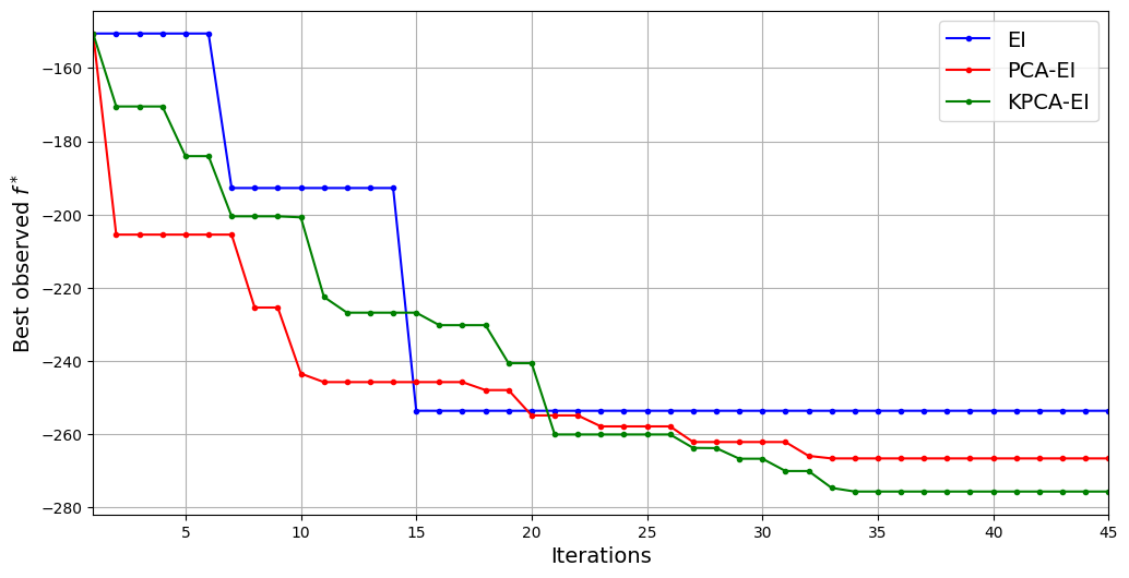
The above plot shows that KPCA-EI can produce a reduction in the best observed value of the function which is greater than both standard EI and PCA-EI. KPCA-EI is able to reduce the best observed value to approximately -275. It is, therefore, the best performing method in this run according to the best observed value of the objective function. However, in this run, it is not as quick as PCA-EI and standard EI to reduce the objective function value. In fact, it can take almost 21 iterations for KPCA-EI to produce a reduction in the objective that is comparable to standard EI and PCA-EI. It is also important to remember that the performance of KPCA-EI depends on the choice of hyperparameters for KPCA which significantly affect the dimensionality reduction and performance of the algorithm.

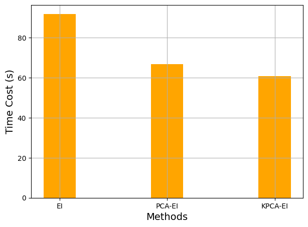
The final block of code below shows the total time cost of each of the sequential sampling algorithms shown in this section. The results show that the use of dimensionality reduction techniques reduces the overall time cost of sequentially sampling a high-dimensional function.

fig, ax = plt.subplots(figsize=(7,5))
methods = ['EI', 'PCA-EI', 'KPCA-EI']
times = [ei_time, pca_time, kpca_time]
ax.bar(methods, times, color ='orange', width = 0.3)
ax.set_xlabel("Methods", fontsize = 14)
ax.set_ylabel("Time Cost (s)", fontsize = 14)
ax.grid()