Constrained Expected Improvement with Probability of Feasibility#
This section demonstrates the probability of feasibility (PF) method which is used for performing balanced exploration and exploitation for constrained optimization problems. The next infill point is obtained by solving an optimization problem, which is written as
where \(PF_i(x)\) is the PF for constraint \(g_i\). It is defined as
where \(G_i\) is the random variable associated with the surrogate model. The \(\hat{g}_i\) and \(\hat{\sigma}_{g,i}\) is the mean prediction and the standard deviation from the constraint surrogate model, respectively. The \(\Phi\) is the cummulative distribution function for the standard normal distribution and \(J\) is the total number of constraints. Essentially, the \(PF_i\) defines the probability that constraint \(g_i\) is less than 0 i.e. the constraint is satisfied. The EI is defined here.
Below code imports required packages, defines modified branin function, constraint, and creates plotting data:
# Imports
import numpy as np
from smt.surrogate_models import KRG
from smt.sampling_methods import LHS, FullFactorial
import matplotlib.pyplot as plt
from pymoo.core.problem import Problem
from pymoo.algorithms.soo.nonconvex.de import DE
from pymoo.optimize import minimize
from pymoo.config import Config
Config.warnings['not_compiled'] = False
from scipy.stats import norm as normal

def modified_branin(x):

    dim = x.ndim

    if dim == 1:
        x = x.reshape(1, -1)

    x1 = x[:,0]
    x2 = x[:,1]

    b = 5.1 / (4*np.pi**2)
    c = 5 / np.pi
    t = 1 / (8*np.pi)

    y = (x2 - b*x1**2 + c*x1 - 6)**2 + 10*(1-t)*np.cos(x1) + 10 + 5*x1

    if dim == 1:
        y = y.reshape(-1)

    return y

def constraint(x):

    dim = x.ndim

    if dim == 1:
        x = x.reshape(1, -1)

    x1 = x[:,0]
    x2 = x[:,1]

    g = -x1*x2 + 30

    if dim == 1:
        g = g.reshape(-1)

    return g

# Bounds
lb = np.array([-5, 0])
ub = np.array([10, 15])

# Plotting data
sampler = FullFactorial(xlimits=np.array( [[lb[0], ub[0]], [lb[1], ub[1]]] ))
num_plot = 400
xplot = sampler(num_plot)
yplot = modified_branin(xplot)
gplot = constraint(xplot)
Differential evolution (DE) from pymoo is used for optimization. Below code defines problem class and initializes DE. Note how problem class computes EI and PF.
# Problem class
class EIPF(Problem):

    def __init__(self, sm_func, sm_const, ymin):
        super().__init__(n_var=2, n_obj=1, n_const=0, xl=lb, xu=ub)

        self.sm_func = sm_func
        self.sm_const = sm_const
        self.ymin = ymin

    def _evaluate(self, x, out, *args, **kwargs):

        # Standard normal
        numerator = self.ymin - self.sm_func.predict_values(x)
        denominator = np.sqrt( self.sm_func.predict_variances(x) )
        z = numerator / denominator

        # EI
        ei = numerator * normal.cdf(z) + denominator * normal.pdf(z)

        # PF
        pf = normal.cdf( - self.sm_const.predict_values(x) / np.sqrt( self.sm_const.predict_variances(x) ) )

        # EI * PF
        # Negative sign because we want to maximize
        out["F"] = - (ei * pf)

# Optimization algorithm
algorithm = DE(pop_size=100, CR=0.8, dither="vector")
Below block of code creates 5 training points and performs sequential sampling process using EI and PF. The maximum number of iterations is set to 20 and a convergence criterion is defined based on maximum value of \(EI\times PF\) obtained in each iteration.
sampler = LHS( xlimits=np.array( [[lb[0], ub[0]], [lb[1], ub[1]]] ), criterion='ese')

# Training data
num_train = 5
xtrain = sampler(num_train)
ytrain = modified_branin(xtrain)
gtrain = constraint(xtrain)

# Variables
itr = 0
max_itr = 20
tol = 1e-3
max_EIPF = [1]
ybest = []
bounds = [(lb[0], ub[0]), (lb[1], ub[1])]
corr = 'squar_exp'
fs = 12

# Sequential sampling Loop
while itr < max_itr and tol < max_EIPF[-1]:

    print("\nIteration {}".format(itr + 1))

    # Initializing the kriging model
    sm_func = KRG(theta0=[1e-2], corr=corr, theta_bounds=[1e-6, 1e2], print_global=False)

    # Initializing the kriging model
    sm_func = KRG(theta0=[1e-2], corr=corr, theta_bounds=[1e-6, 1e2], print_global=False)
    sm_const = KRG(theta0=[1e-2], corr=corr, theta_bounds=[1e-6, 1e2], print_global=False)

    # Setting the training values
    sm_func.set_training_values(xtrain, ytrain)
    sm_const.set_training_values(xtrain, gtrain)

    # Creating surrogate model
    sm_func.train()
    sm_const.train()

    # Find the best feasible sample
    ybest.append(np.min(ytrain[gtrain < 0]))
    index = np.where(ytrain == ybest[-1])[0][0]

    # Find the minimum of surrogate model
    result = minimize(EIPF(sm_func, sm_const, ybest[-1]), algorithm, verbose=False)

    # Computing true function value at infill point
    y_infill = modified_branin(result.X.reshape(1,-1))

    # Storing variables
    if itr == 0:
        max_EIPF[0] = -result.F[0]
        xbest = xtrain[index,:].reshape(1,-1)
    else:
        max_EIPF.append(-result.F[0])
        xbest = np.vstack((xbest, xtrain[index,:]))

    print("Maximum EI*PF: {}".format(max_EIPF[-1]))
    print("Best observed value: {}".format(ybest[-1]))

    # Appending the the new point to the current data set
    xtrain = np.vstack(( xtrain, result.X.reshape(1,-1) ))
    ytrain = np.append( ytrain, y_infill )
    gtrain = np.append( gtrain, constraint(result.X.reshape(1,-1)) )

    itr = itr + 1 # Increasing the iteration number

# Printing the final results
print("\nBest feasible point:")
print("x*: {}".format(xbest[-1]))
print("f*: {}".format(ybest[-1]))
print("g*: {}".format(gtrain[index]))
Iteration 1
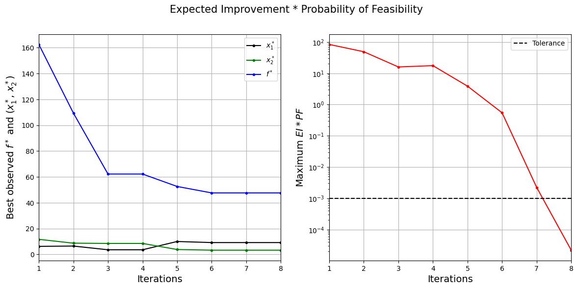
Maximum EI*PF: 83.46479227981871
Best observed value: 162.44754405214525

Iteration 2
Maximum EI*PF: 48.78667259537681
Best observed value: 109.31174558873258

Iteration 3
Maximum EI*PF: 15.88913593522882
Best observed value: 62.178604305154806

Iteration 4
Maximum EI*PF: 17.512329130215438
Best observed value: 62.178604305154806

Iteration 5
Maximum EI*PF: 3.86193941020984
Best observed value: 52.57079769357797

Iteration 6
Maximum EI*PF: 0.543261589600655
Best observed value: 47.58123449309893

Iteration 7
Maximum EI*PF: 0.0022347763277108315
Best observed value: 47.58123449309893

Iteration 8
Maximum EI*PF: 2.1885959627193973e-05
Best observed value: 47.58123449309893

Best feasible point:
x*: [9.16168372 3.28403339]
f*: 47.58123449309893
g*: -0.0872752292702863
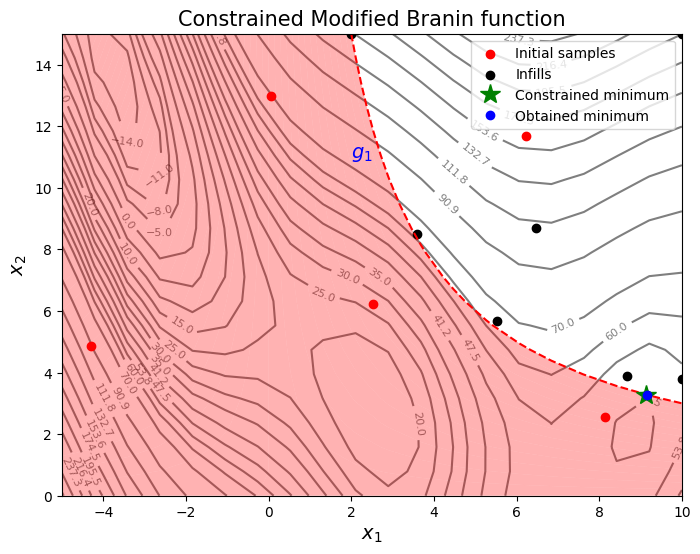
NOTE: The minimum obtained at the end of process is the minimum feasible \(y\) observed in the training data and not the minimum of the surrogate model.
Below block of code plots the convergence of best observed value and \(EI\times PF\).
####################################### Plotting convergence history

fig, ax = plt.subplots(1, 2, figsize=(14,6))
ax[0].plot(np.arange(itr) + 1, xbest[:,0], c="black", label='$x_1^*$', marker=".")
ax[0].plot(np.arange(itr) + 1, xbest[:,1], c="green", label='$x_2^*$', marker=".")
ax[0].plot(np.arange(itr) + 1, ybest, c="blue", label='$f^*$', marker=".")
ax[0].set_xlabel("Iterations", fontsize=14)
ax[0].set_ylabel("Best observed $f^*$ and ($x_1^*$, $x_2^*$)", fontsize=14)
ax[0].legend()
ax[0].set_xlim(left=1, right=itr)
ax[0].grid()

ax[1].plot(np.arange(itr) + 1, max_EIPF, c="red", marker=".")
ax[1].plot(np.arange(itr) + 1, [tol]*(itr), c="black", linestyle="--", label="Tolerance")
ax[1].set_xlabel("Iterations", fontsize=14)
ax[1].set_ylabel("Maximum $EI*PF$", fontsize=14)
ax[1].set_xlim(left=1, right=itr)
ax[1].grid()
ax[1].legend()
ax[1].set_yscale("log")

fig.suptitle("Expected Improvement * Probability of Feasibility", fontsize=15)
Text(0.5, 0.98, 'Expected Improvement * Probability of Feasibility')

The figure on the left shows the history of best feasible \(y\) value and the corresponding \(x\) values, and figure on the right shows the convergence of \(EI\times PF\). At start, the value of \(EI\times PF\) is high since the amount of possible improvement over the current best feasible point is high. As the iterations progress, the best feasible value reaches the global minimum and the \(EI\times PF\) decreases. Also, note that process stopped before reaching maximum number of infills since the convergence criteria was met.
Below code plots the infill points.
####################################### Plotting initial samples and infills

# Reshaping into grid
reshape_size = int(np.sqrt(num_plot))
X = xplot[:,0].reshape(reshape_size, reshape_size)
Y = xplot[:,1].reshape(reshape_size, reshape_size)
Z = yplot.reshape(reshape_size, reshape_size)
G = gplot.reshape(reshape_size, reshape_size)

# Level
levels = np.linspace(-17, -5, 5)
levels = np.concatenate((levels, np.linspace(0, 30, 7)))
levels = np.concatenate((levels, np.linspace(35, 60, 5)))
levels = np.concatenate((levels, np.linspace(70, 300, 12)))

fig, ax = plt.subplots(figsize=(8,6))

# Plot function
CS=ax.contour(X, Y, Z, levels=levels, colors='k', linestyles='solid', alpha=0.5, zorder=-10)
ax.clabel(CS, inline=1, fontsize=8)

# Plot constraint
ax.contour(X, Y, G, levels=[0], colors='r', linestyles='dashed')
ax.contourf(X, Y, G, levels=np.linspace(0,G.max()), colors="red", alpha=0.3, antialiased = True)
ax.annotate('$g_1$', xy =(2.0, 11.0), fontsize=14, color='b')

# Plot minimum
ax.scatter(xtrain[0:num_train,0], xtrain[0:num_train,1], c="red", label='Initial samples')
ax.scatter(xtrain[num_train:,0], xtrain[num_train:,1], c="black", label='Infills')
ax.plot(9.143, 3.281, 'g*', markersize=15, label="Constrained minimum")
ax.plot(xtrain[index,0], xtrain[index,1], 'bo', label="Obtained minimum")

# Asthetics
ax.set_xlabel("$x_1$", fontsize=14)
ax.set_ylabel("$x_2$", fontsize=14)
ax.set_title("Constrained Modified Branin function", fontsize=15)
ax.legend()
<matplotlib.legend.Legend at 0x70ab1ef147c0>

From the above plots, it can be seen that EI and PF finds the minimum of the modified branin function while balancing exploration and exploitation.
NOTE: Due to randomness in differential evolution, results may vary slightly between runs. So, it is recommended to run the code multiple times to see average behavior.
Final result:
Parameter |
True minimum |
Obtained minimum |
|---|---|---|
\(x_1^*\) |
9.143 |
9.162 |
\(x_2^*\) |
3.281 |
3.284 |
\(f(x_1^*, x_2^*)\) |
47.560 |
47.581 |
\(g_1(x_1^*, x_2^*)\) |
0.0 |
-8.728 \(\cdot 10^{-2}\) |